dichasus-0d5x Dataset: Distributed Arrays: Indoor LoS, Lab Room
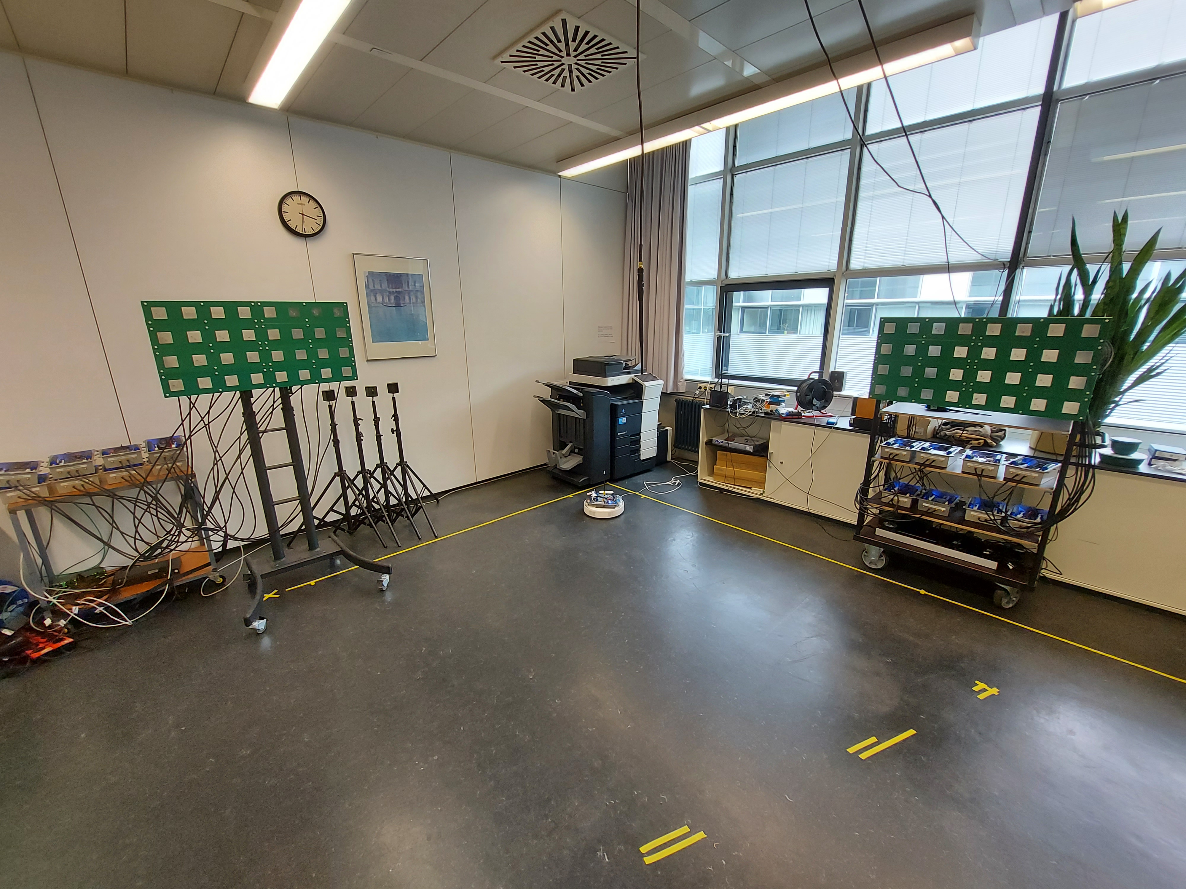
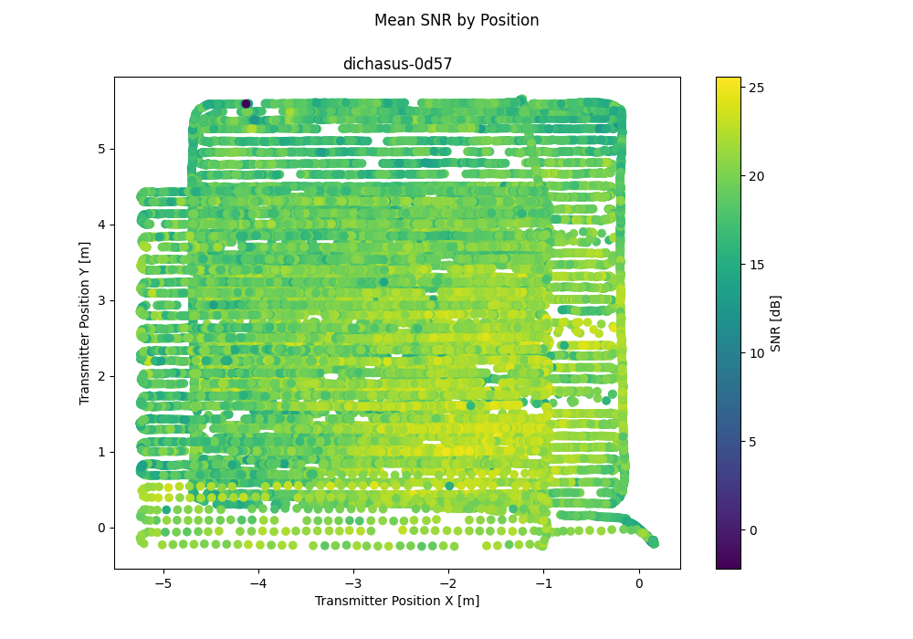
Distributed measurement with two separate antenna arrays in an indoor lab room. Mostly line-of-sight dataset with vacuum robot-mounted transmitter.
50.000 MHz
Signal Bandwidth
1024
OFDM Subcarriers
162462
Data Points
9483.6 s
Total Duration
42.7 GB
Total Download Size
32
Number of Antennas
Indoor
Type of Environment
1.272000 GHz
Carrier Frequency
Distributed
Antenna Setup
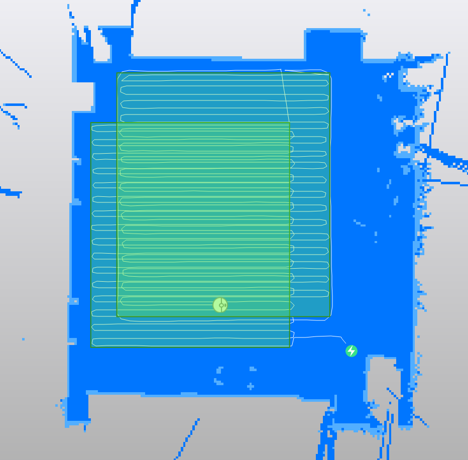
2D LiDAR
Position-Tagged
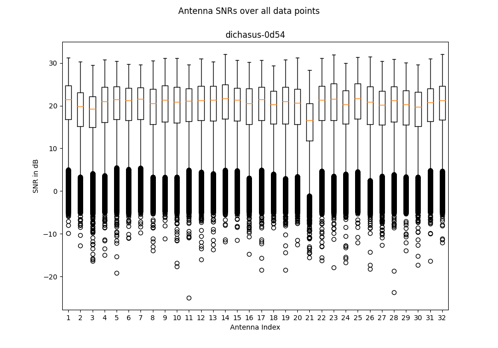
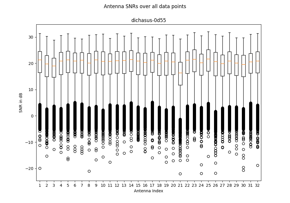
Experiment Setup
Data Analysis
Warnings
Antenna Configuration
Antenna 1: Antenna array near wall
| 31 | 29 | 0 | 13 | 1 | 12 | 3 | 7 |
| 30 | 26 | 21 | 25 | 22 | 15 | 24 | 8 |
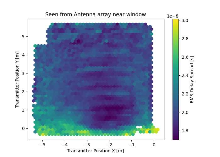
Antenna 2: Antenna array near window
| 28 | 5 | 10 | 14 | 6 | 2 | 16 | 18 |
| 19 | 4 | 23 | 17 | 20 | 11 | 9 | 27 |
Python: Import with TensorFlow
#!/usr/bin/env python3
import tensorflow as tf
raw_dataset = tf.data.TFRecordDataset(["tfrecords/dichasus-0d51.tfrecords", "tfrecords/dichasus-0d52.tfrecords", "tfrecords/dichasus-0d53.tfrecords", "tfrecords/dichasus-0d54.tfrecords", "tfrecords/dichasus-0d55.tfrecords", "tfrecords/dichasus-0d56.tfrecords", "tfrecords/dichasus-0d57.tfrecords"])
feature_description = {
"cfo": tf.io.FixedLenFeature([], tf.string, default_value = ''),
"csi": tf.io.FixedLenFeature([], tf.string, default_value = ''),
"gt-interp-age-lidar": tf.io.FixedLenFeature([], tf.float32, default_value = 0),
"pos-lidar": tf.io.FixedLenFeature([], tf.string, default_value = ''),
"rot-lidar": tf.io.FixedLenFeature([], tf.float32, default_value = 0),
"snr": tf.io.FixedLenFeature([], tf.string, default_value = ''),
"time": tf.io.FixedLenFeature([], tf.float32, default_value = 0),
}
def record_parse_function(proto):
record = tf.io.parse_single_example(proto, feature_description)
# Measured carrier frequency offset between MOBTX and each receive antenna.
cfo = tf.ensure_shape(tf.io.parse_tensor(record["cfo"], out_type = tf.float32), (32))
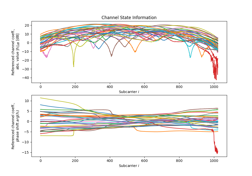
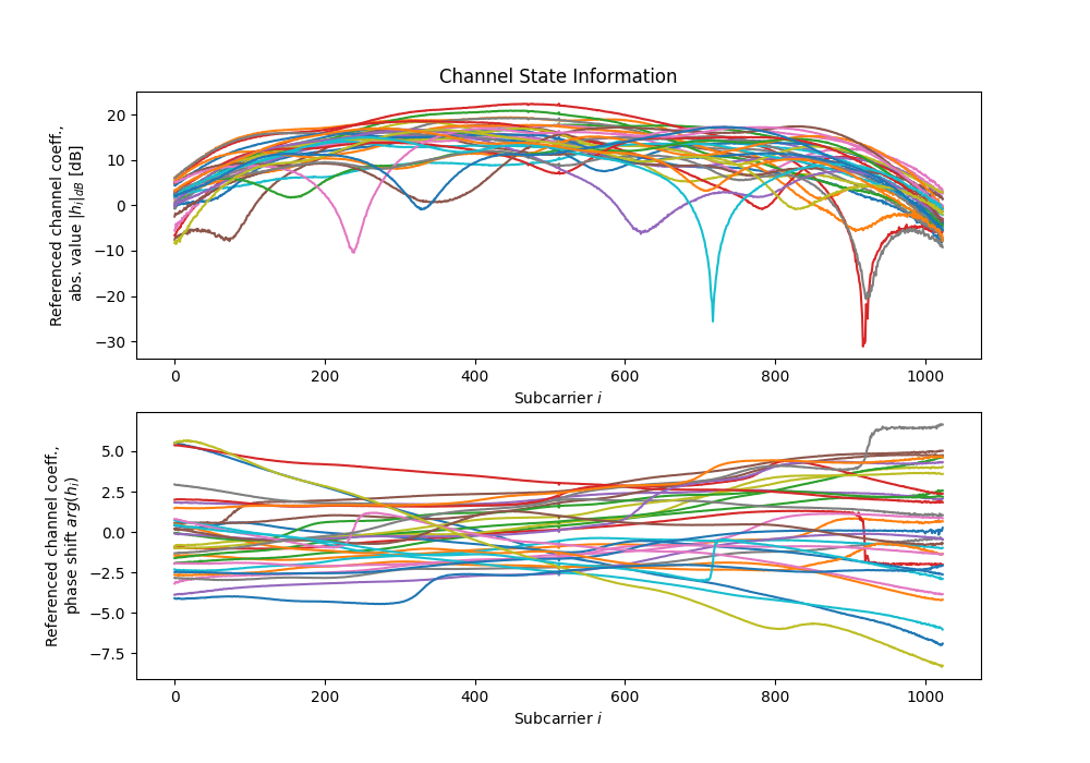
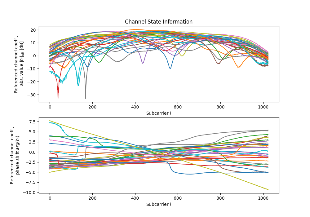
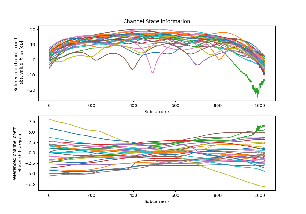
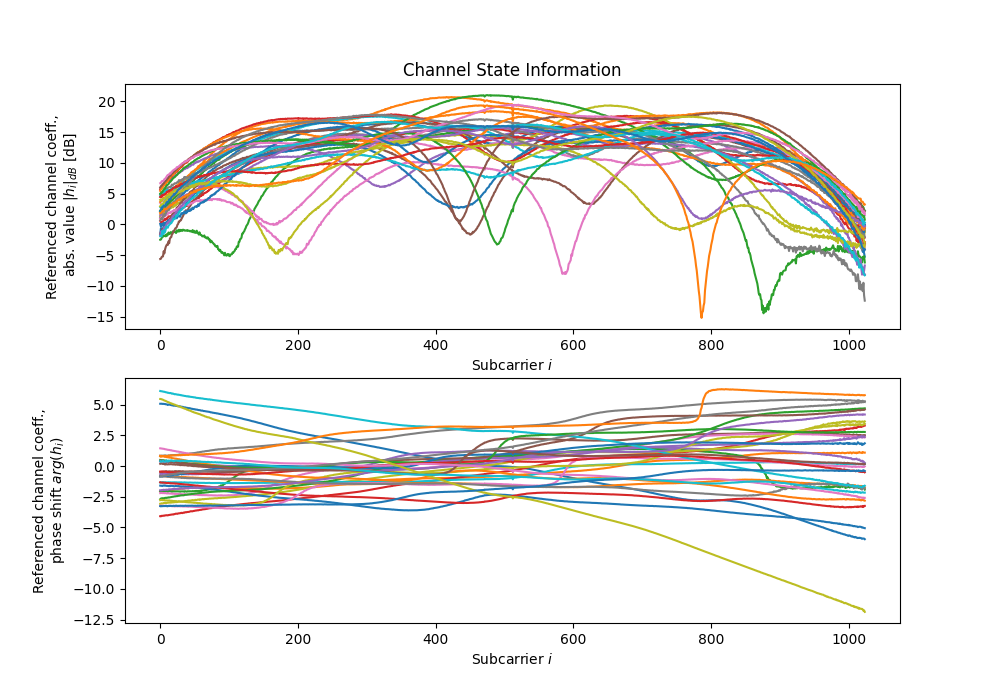
# Channel coefficients for all antennas, over all subcarriers, real and imaginary parts
csi = tf.ensure_shape(tf.io.parse_tensor(record["csi"], out_type = tf.float32), (32, 1024, 2))
# Time in seconds to closest known LiDAR position. Indicates quality of linear interpolation.
gt_interp_age_lidar = tf.ensure_shape(record["gt-interp-age-lidar"], ())
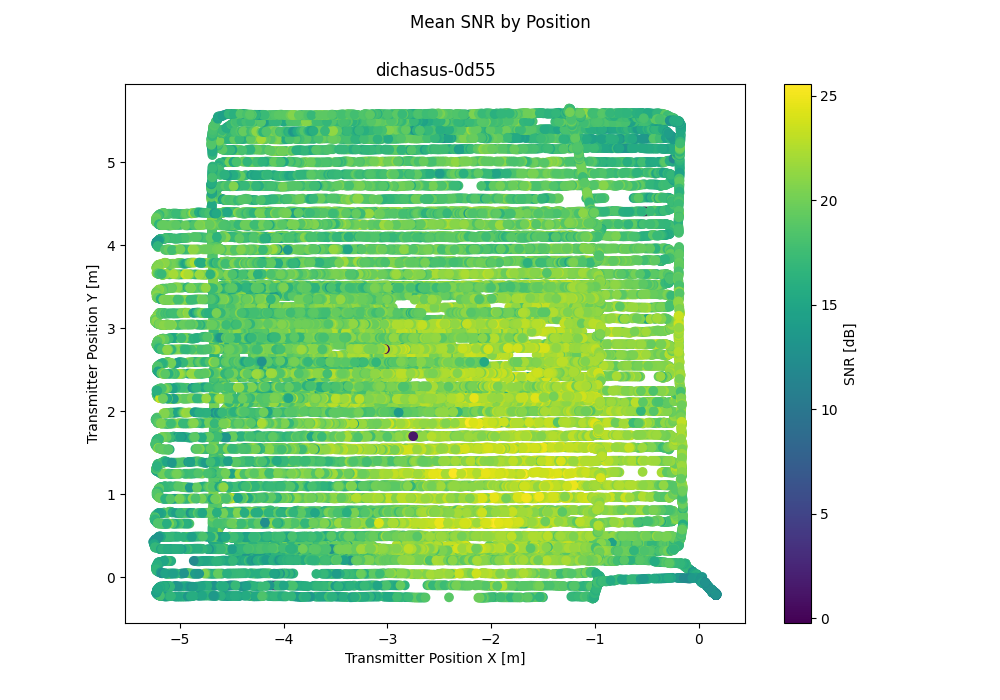
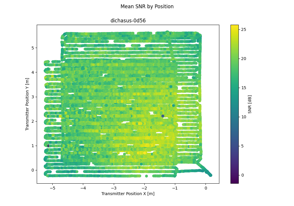
# Position of transmitter determined by vacuum robot LiDAR, in meters (X / Y coordinates)
pos_lidar = tf.ensure_shape(tf.io.parse_tensor(record["pos-lidar"], out_type = tf.float64), (2))
# Rotation of robot relative to its initial parking position, in radians
rot_lidar = tf.ensure_shape(record["rot-lidar"], ())
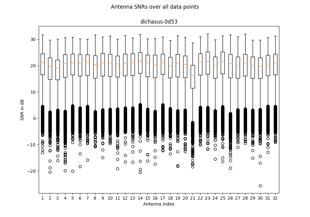
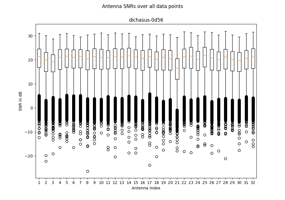
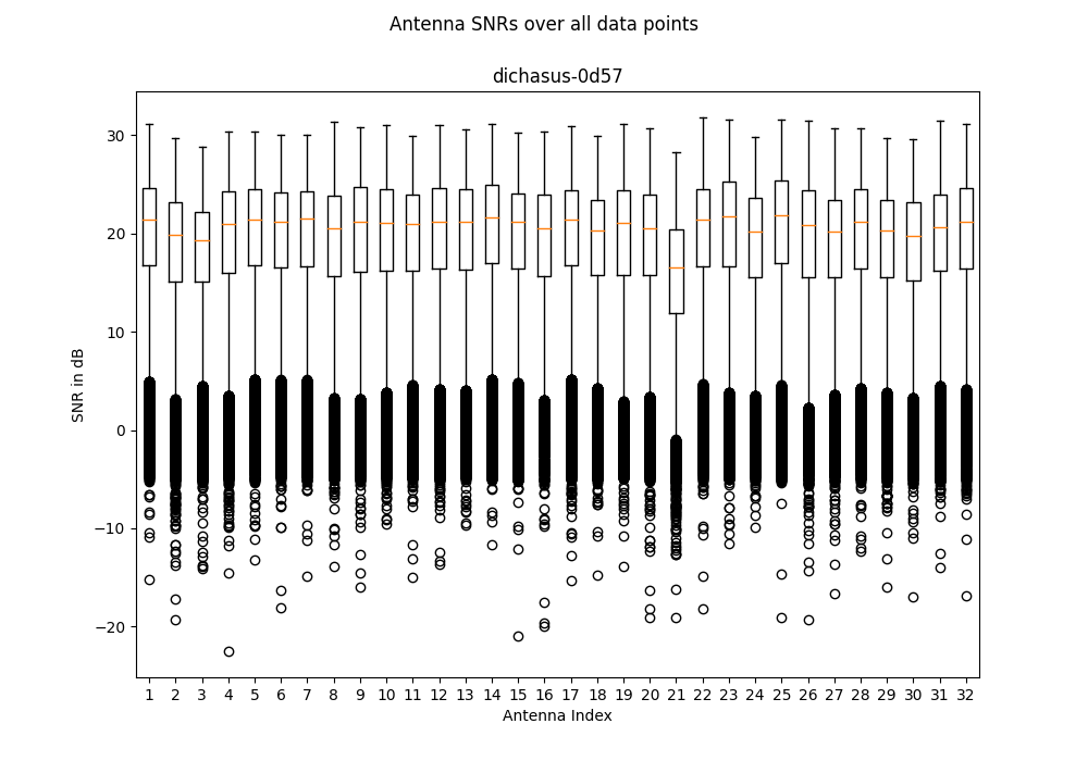
# Signal-to-Noise ratio estimates for all antennas
snr = tf.ensure_shape(tf.io.parse_tensor(record["snr"], out_type = tf.float32), (32))
# Timestamp since start of measurement campaign, in seconds
time = tf.ensure_shape(record["time"], ())
return cfo, csi, gt_interp_age_lidar, pos_lidar, rot_lidar, snr, time
dataset = raw_dataset.map(record_parse_function, num_parallel_calls = tf.data.experimental.AUTOTUNE)
# Optional: Cache dataset in RAM for faster training
dataset = dataset.cache()How to Cite
Please refer to the home page for information on how to cite any of our datasets in your research. For this dataset in particular, you may use the following BibTeX:
@data{dataset-dichasus-0d5x,
	author    = {Euchner, Florian and Gauger, Marc},
	publisher = {DaRUS},
	title     = {{CSI Dataset dichasus-0d5x: Distributed Arrays: Indoor LoS, Lab Room}},
	doi       = {doi:10.18419/darus-2218},
	url       = {https://doi.org/doi:10.18419/darus-2218},
	year      = {2021}
}
Download
This dataset consists of 7 files. Descriptions of these files as well as download links are provided below.
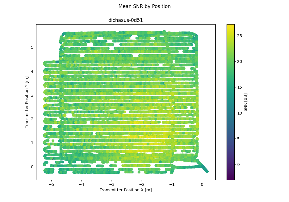
dichasus-0d51
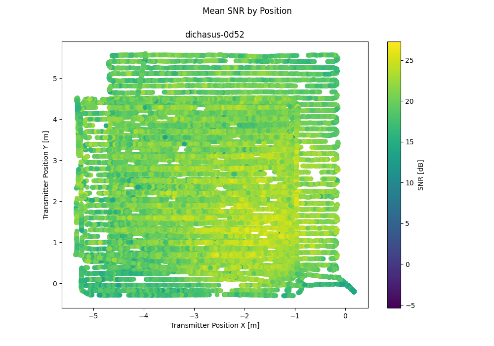
dichasus-0d52

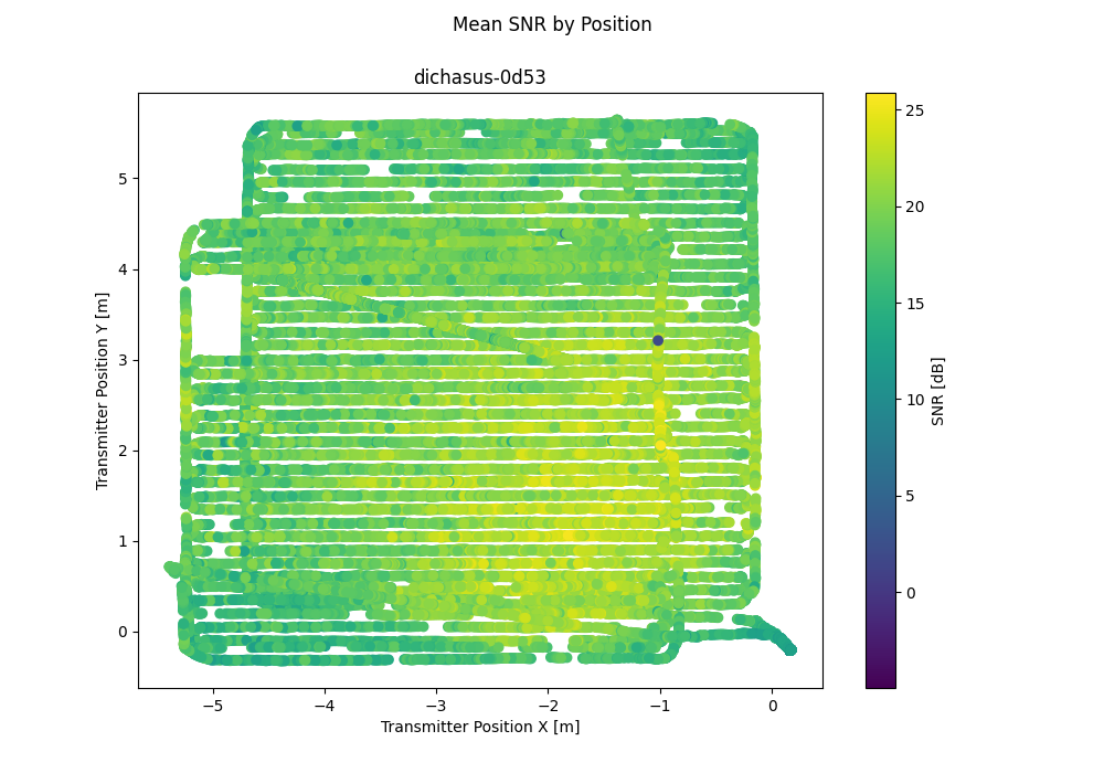
dichasus-0d53

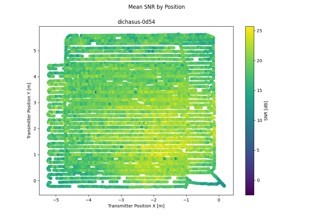
dichasus-0d54
dichasus-0d55
dichasus-0d56
Derived Channel Statistics
Channel statistics such as delay spread, k-Factor and path loss exponent are a good way to characterize a wireless channel measurement and to parametrize a channel model. Using estimation algorithms contributed by Janina Sanzi, we automatically extract the following channel statistics from the measured datasets:
RMS Delay Spread
The delay spread of a wireless channel is inversely proportional to the channel's coherence bandwidth and indicates how "spread out" the lengths of the various multipath propagation paths are. For every datapoint, the delay spread can be characterized by its root mean square value and the resulting delay spreads can be plotted over the measurement area: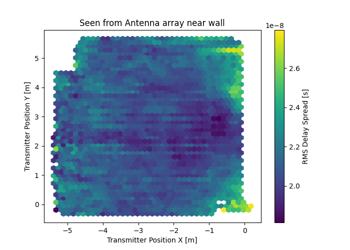
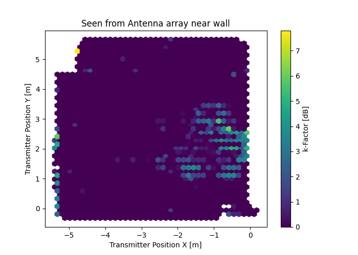
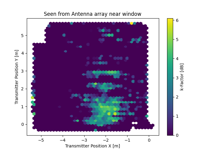
Rician K-Factor
The Rician K-factor is defined as the power ratio between dominant and diffuse component, usually expressed in decibels. We estimate the K-factor with a moment-method based on the distribution of of channel coefficient powers. The resulting K-Factors be plotted over the measurement area: