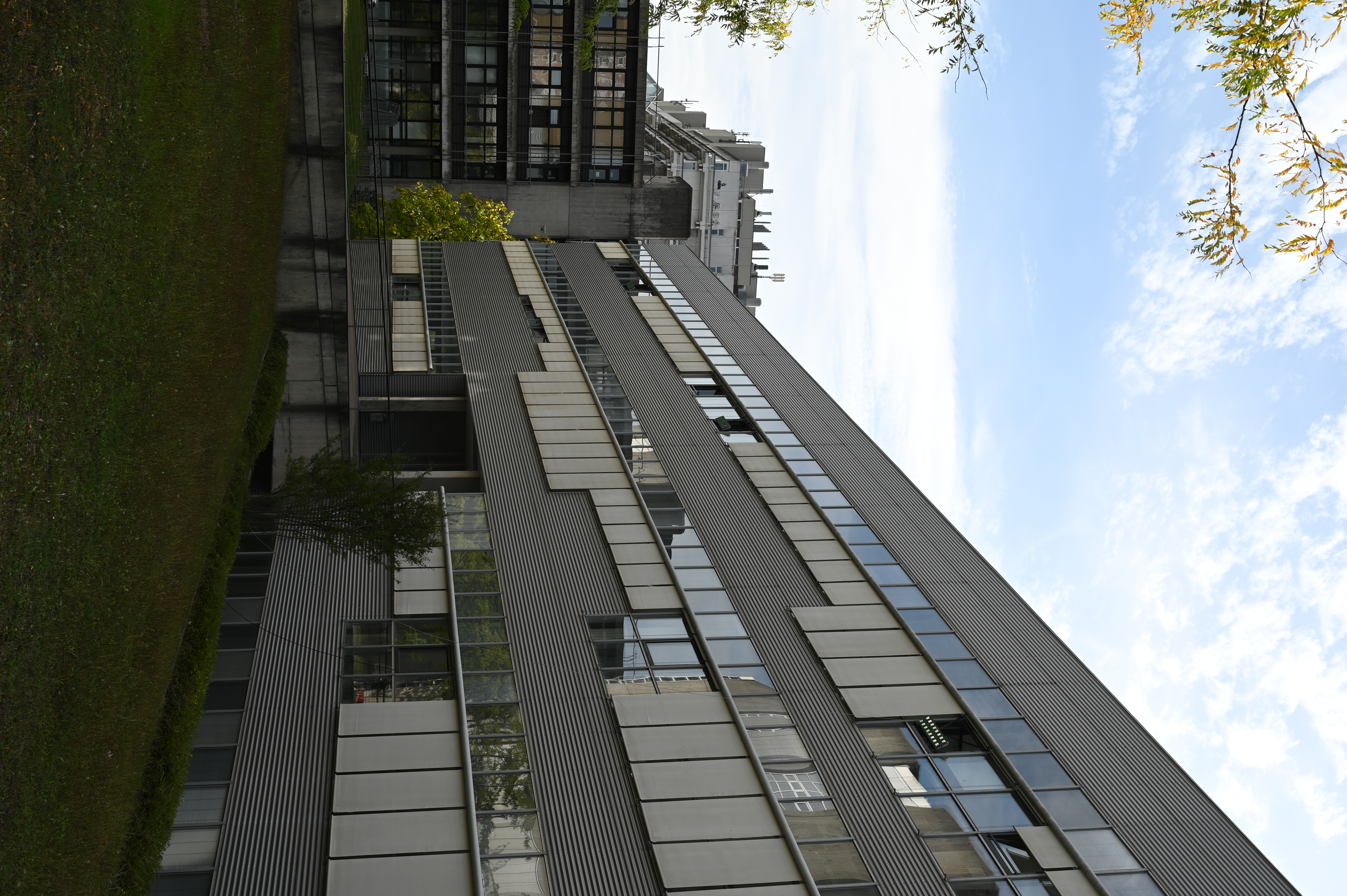
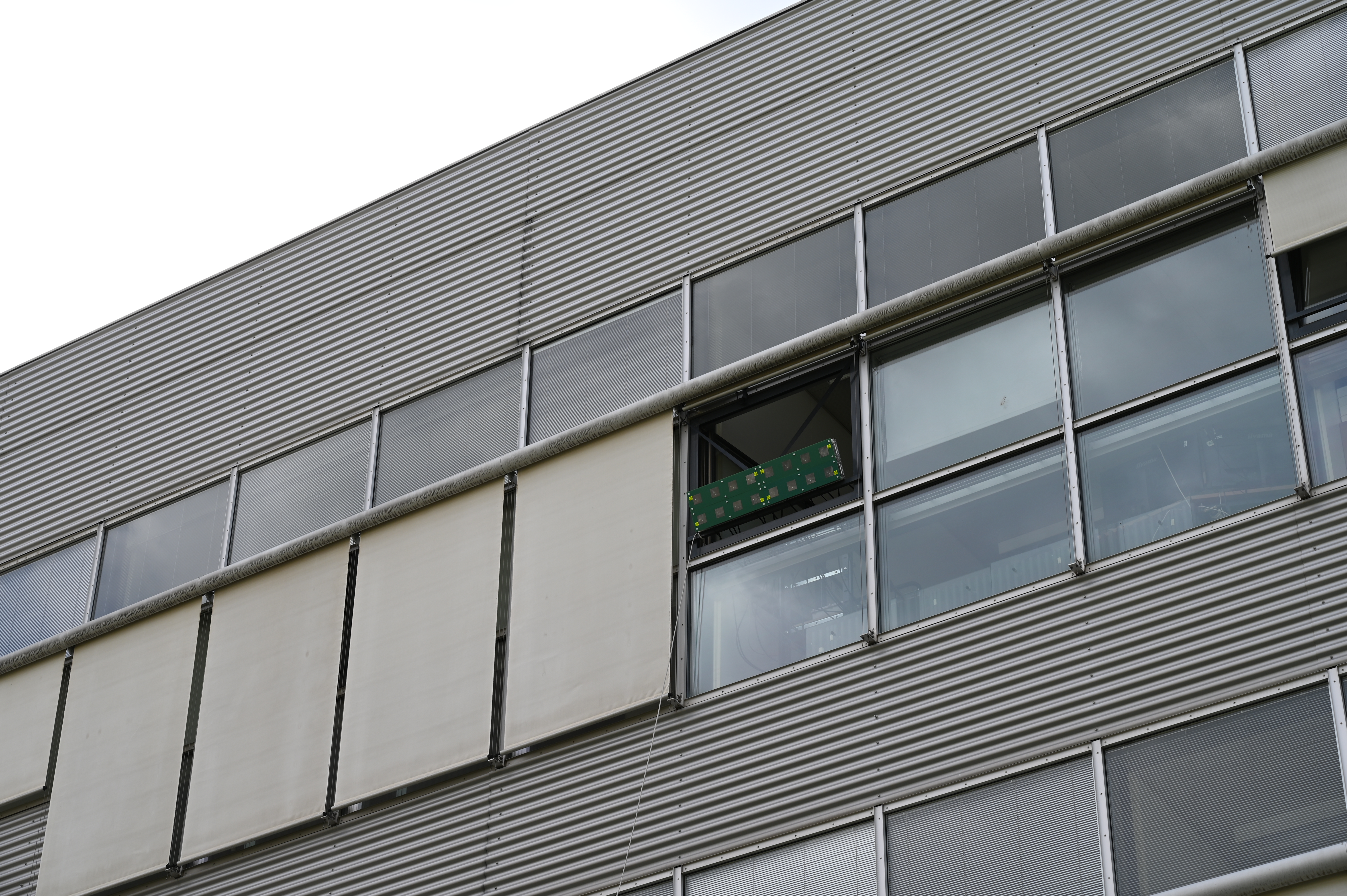
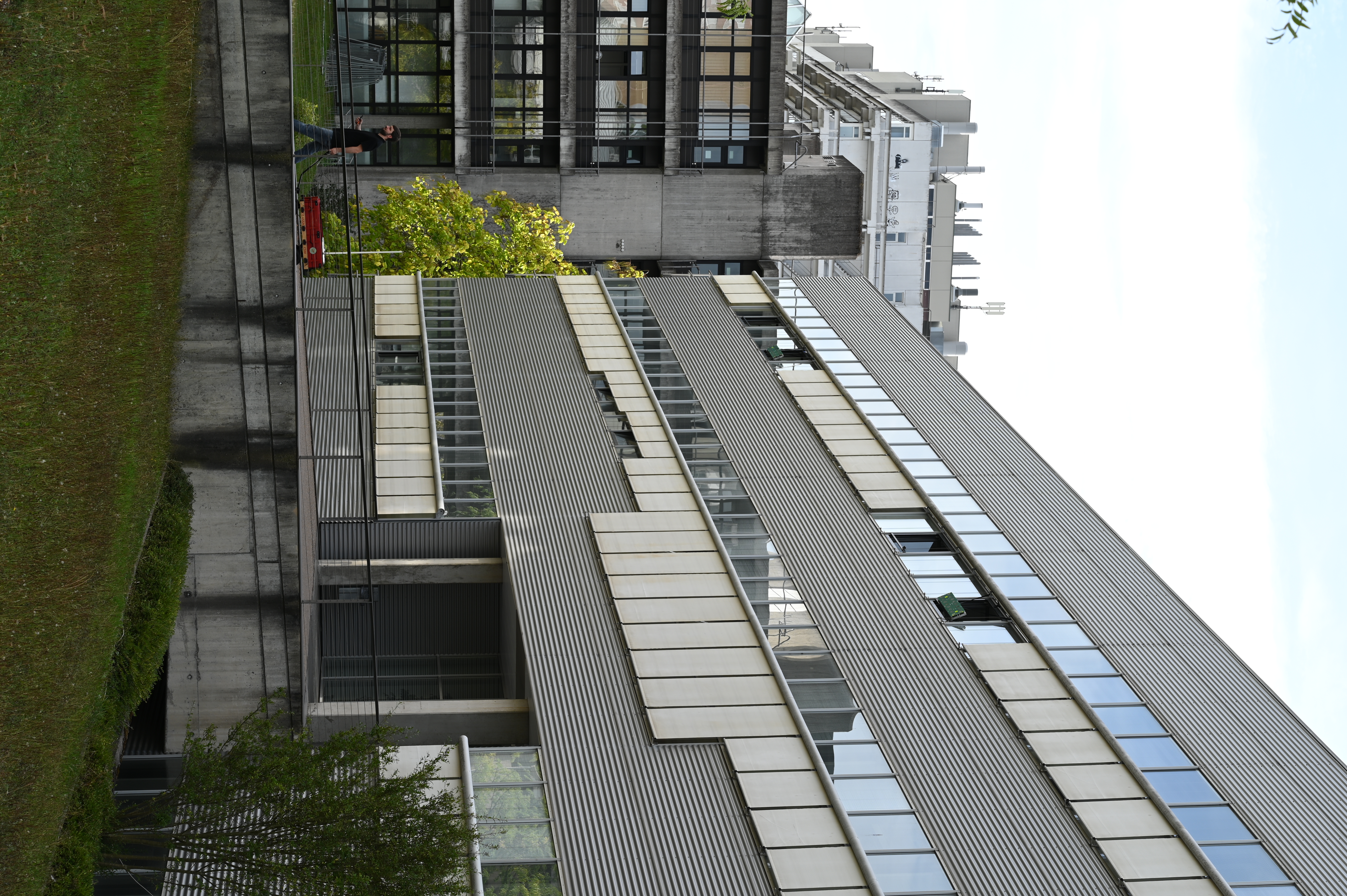
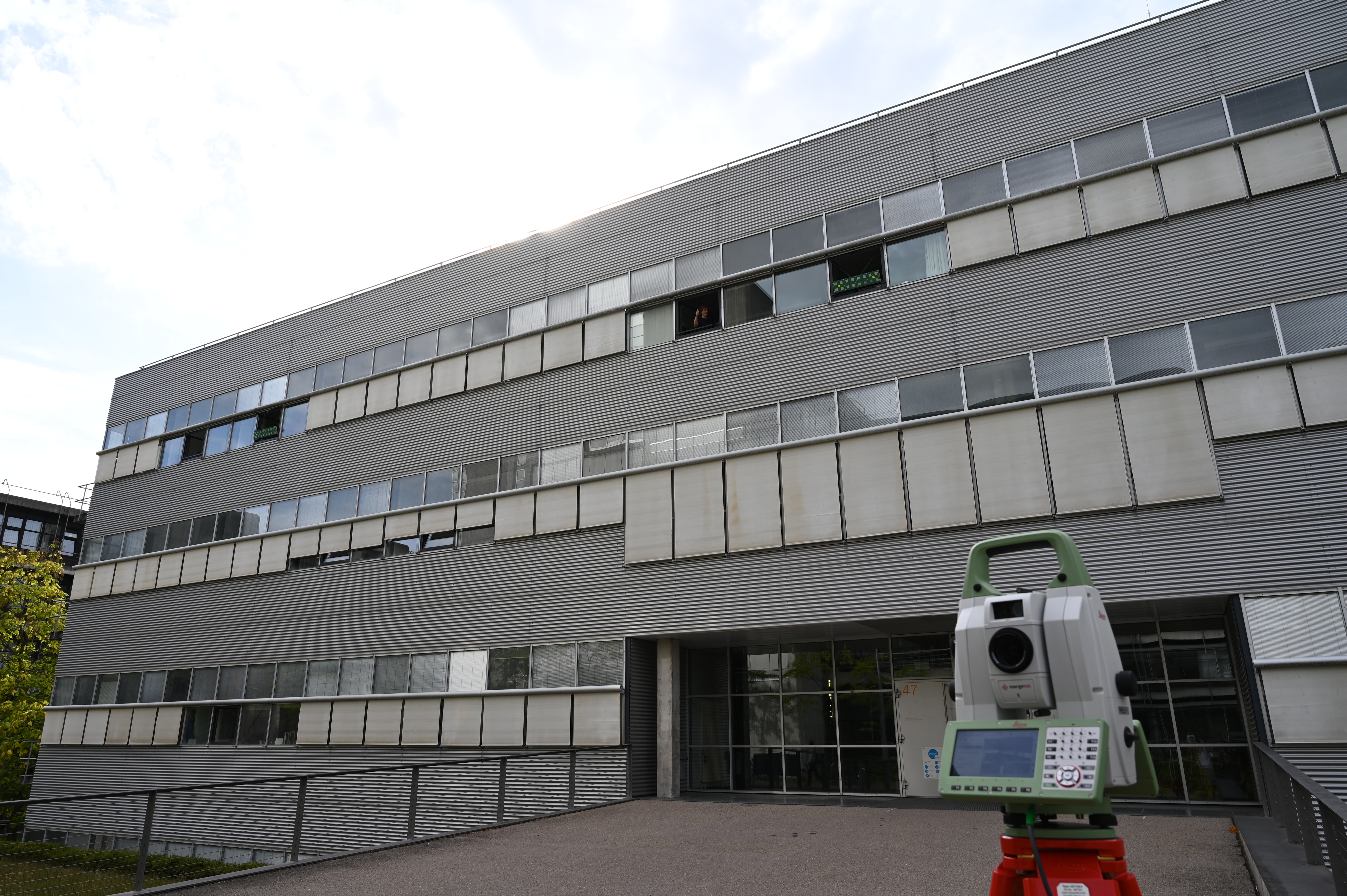
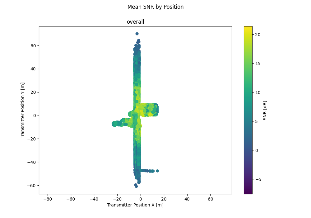
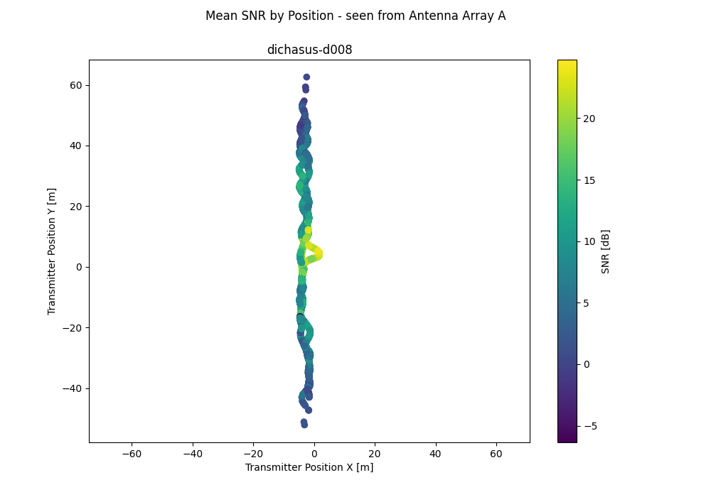
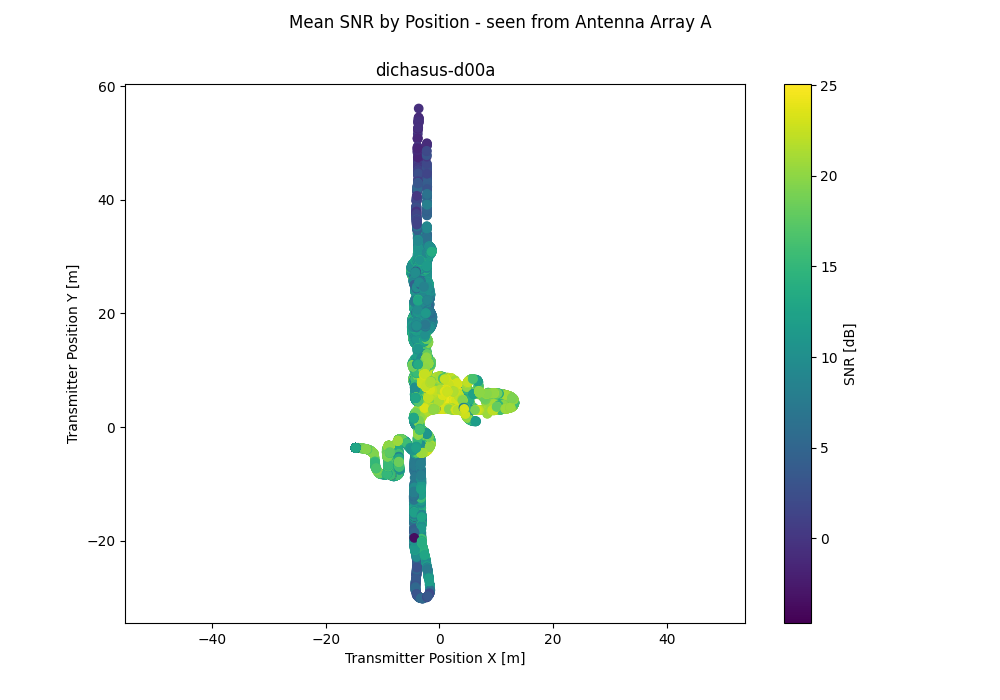
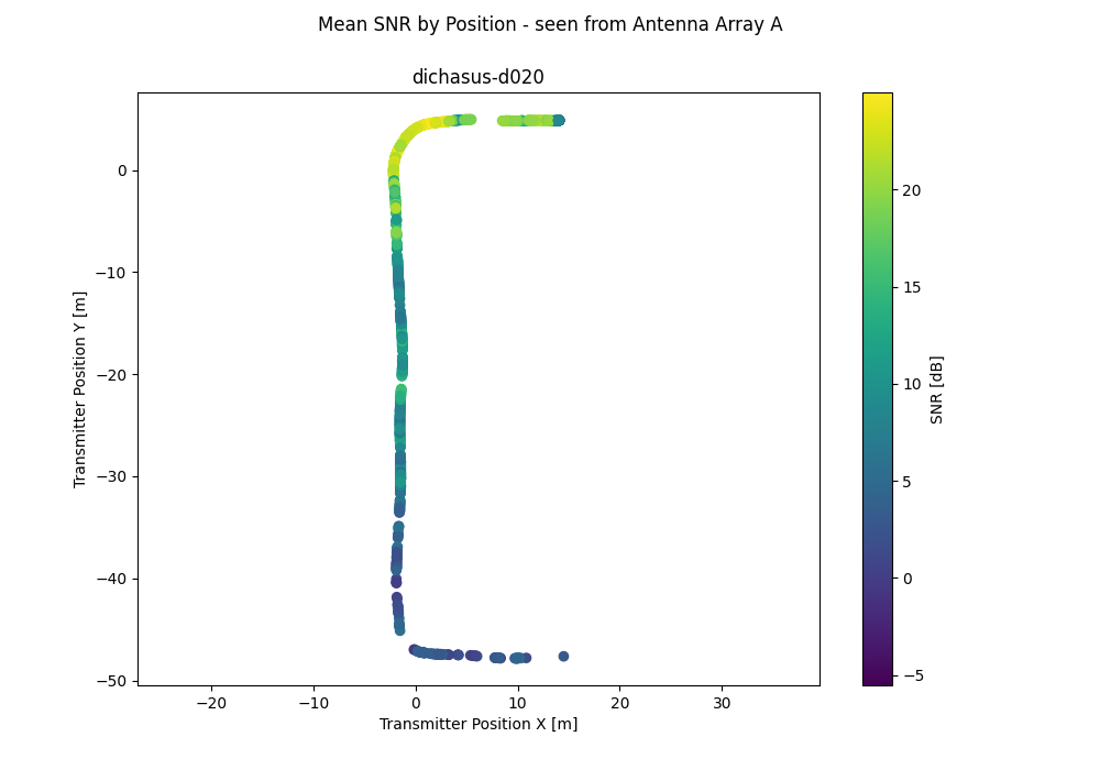
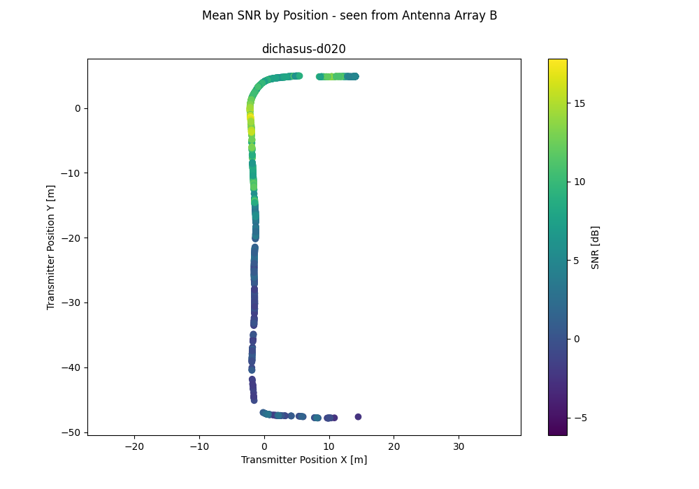
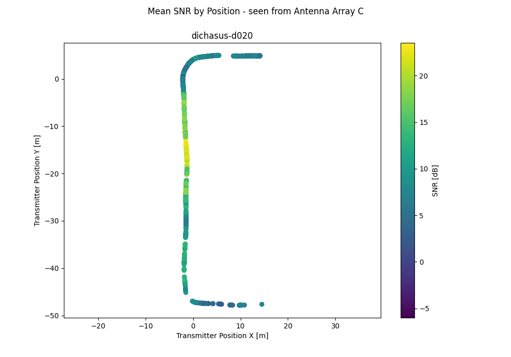
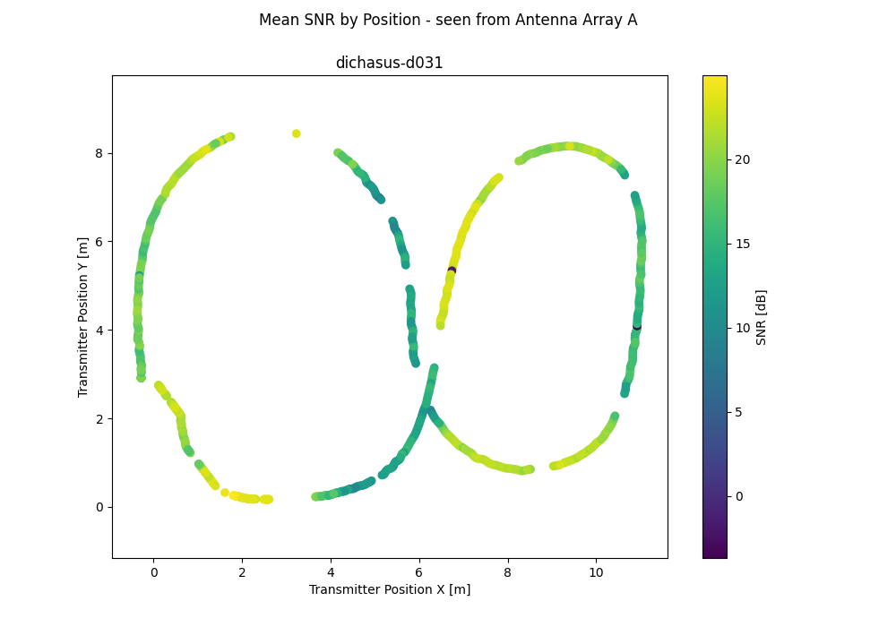
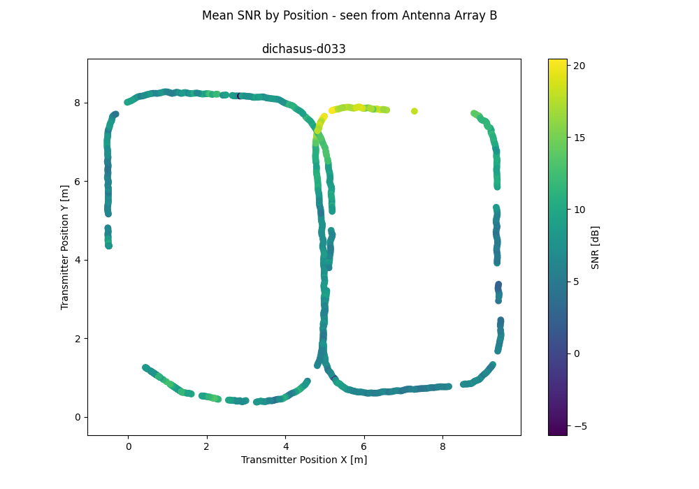
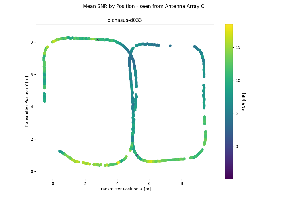
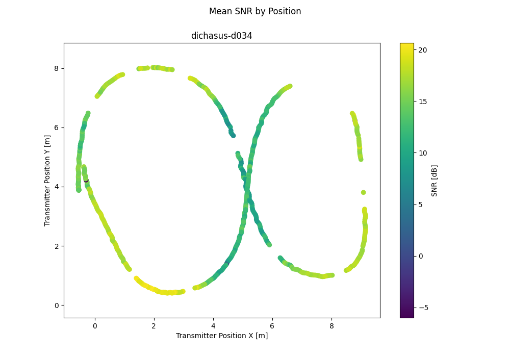
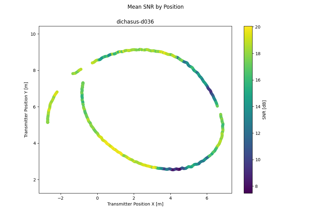
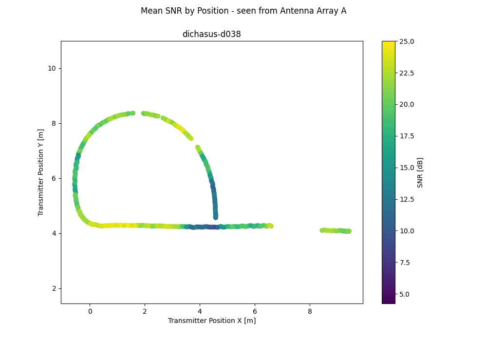
dichasus-dxxx-reduced Dataset: Outdoor - Three arrays distributed along the facade (one antenna removed)
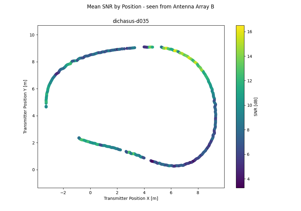
Three 2 x 8 antenna arrays are distributed along the facade of a building, separated by up to 35m (one antenna less due to synchronization issues).
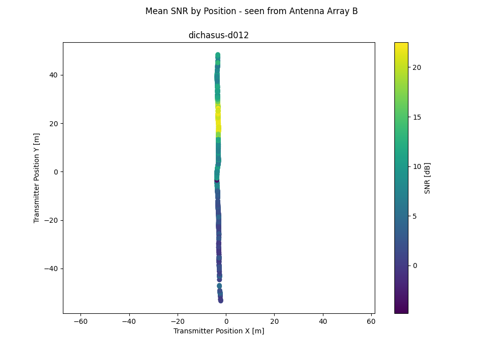
This dataset is generated from the same recording as dichasus-dxxx-complete. However, due to the fact that one antenna that is part of array B was not perfectly reliable because of synchronization issues, that antenna was removed from this dataset. This reduces the number of antennas by one, but increases the number of valid collected datapoints since datapoints that previously had to be rejected due to bad synchronization at that one antenna are now also part of the dataset. This dataset therefore contains more trajectories and datapoints than dichasus-dxxx-complete, but is otherwise identical.
50.000 MHz
Signal Bandwidth
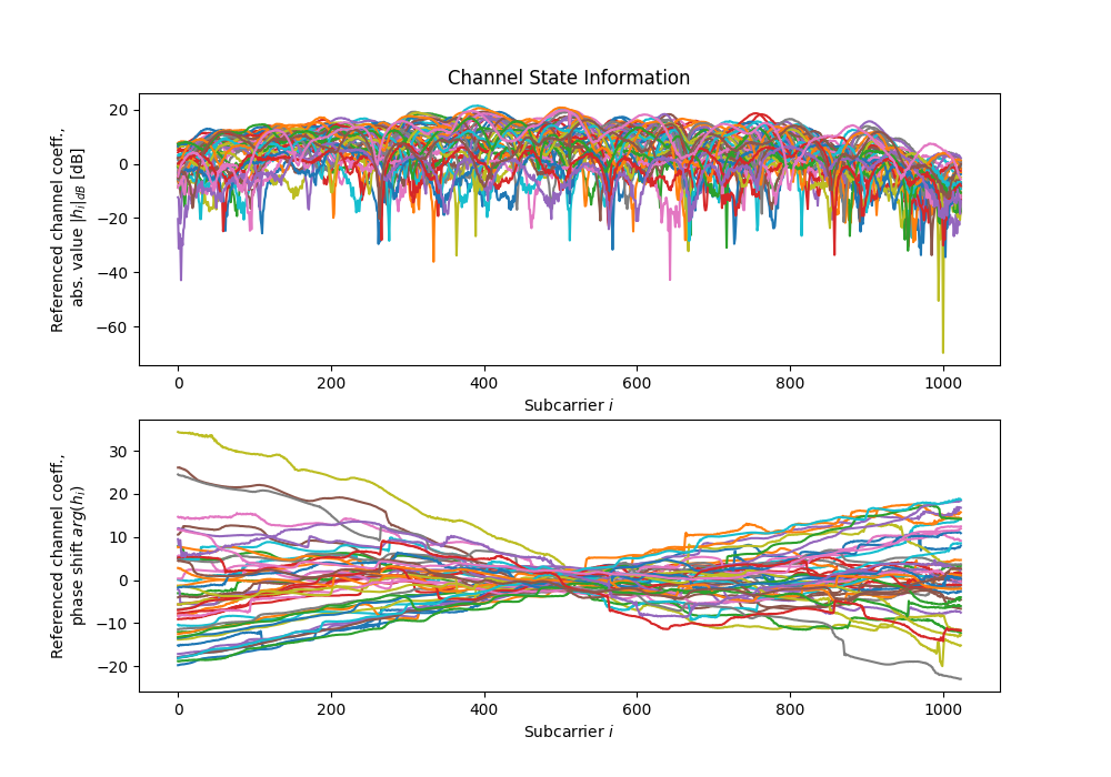
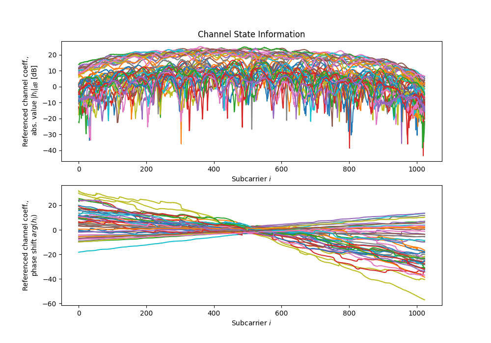
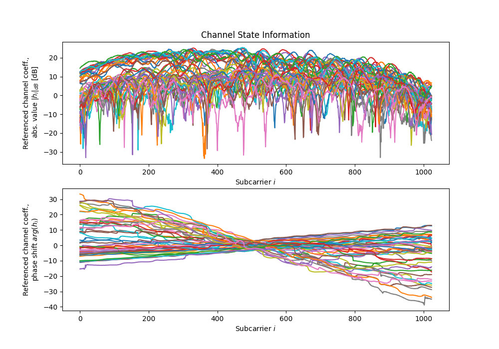
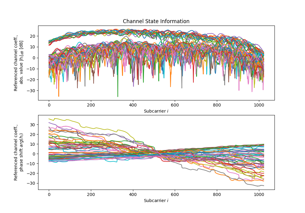
1024
OFDM Subcarriers
113709
Data Points
7865.5 s
Total Duration
43.8 GB
Total Download Size
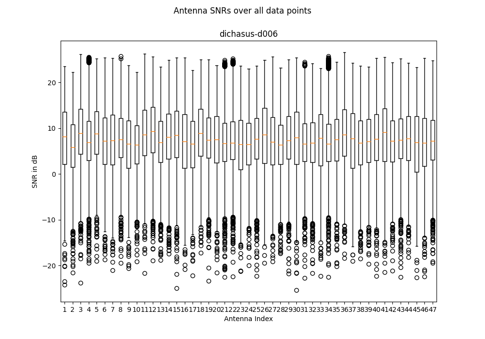
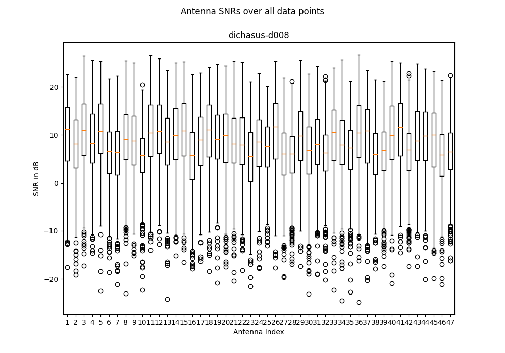
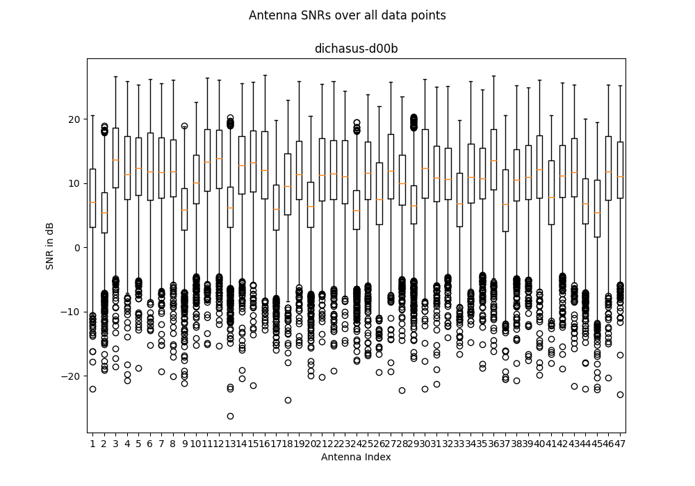
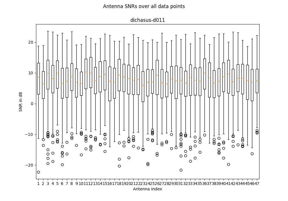
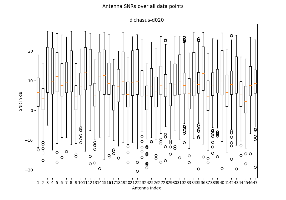
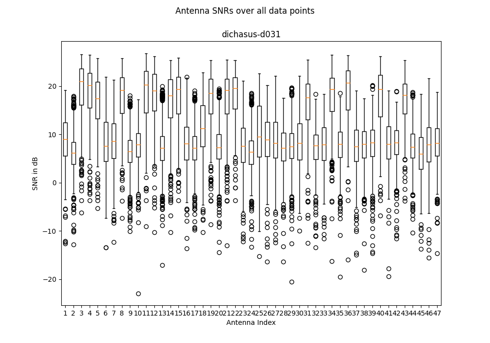
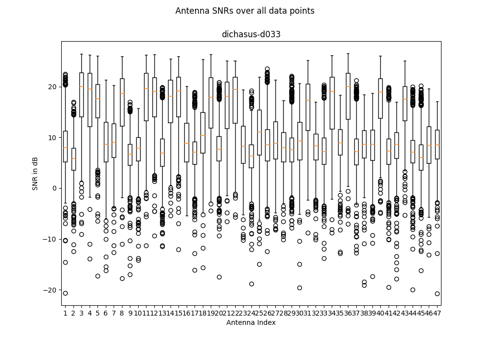
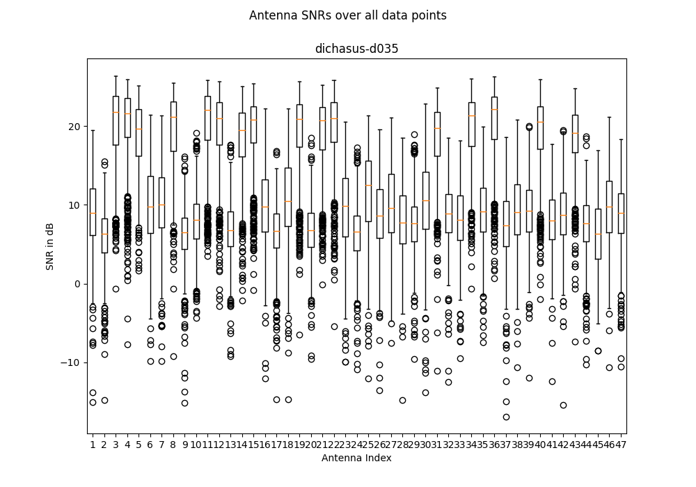
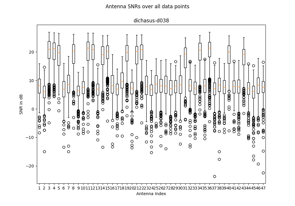
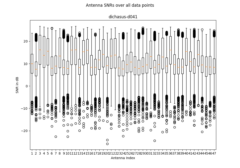
47
Number of Antennas
Outdoor
Type of Environment
1.272000 GHz
Carrier Frequency
Distributed
Antenna Setup
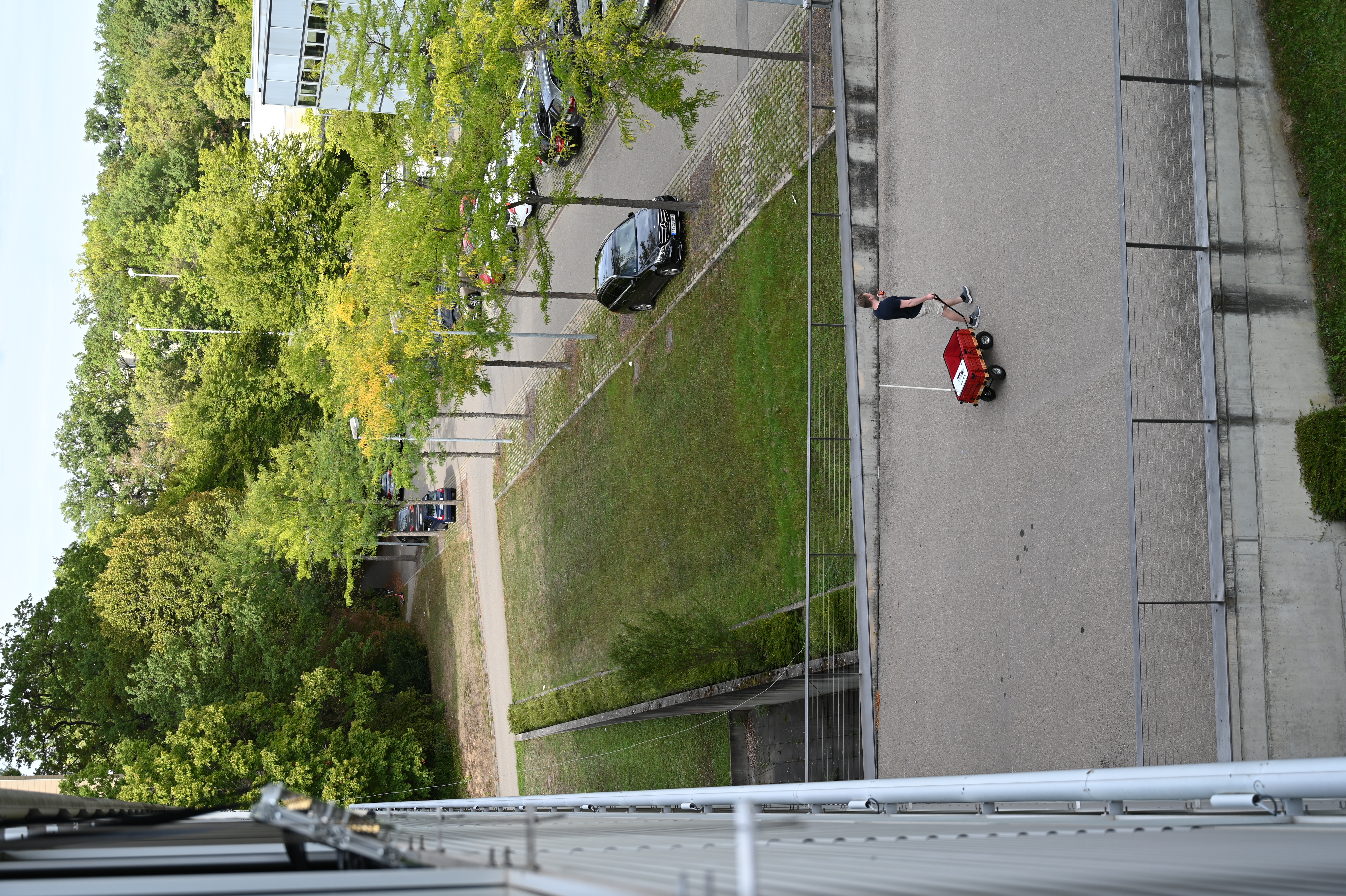
3D Tachymeter
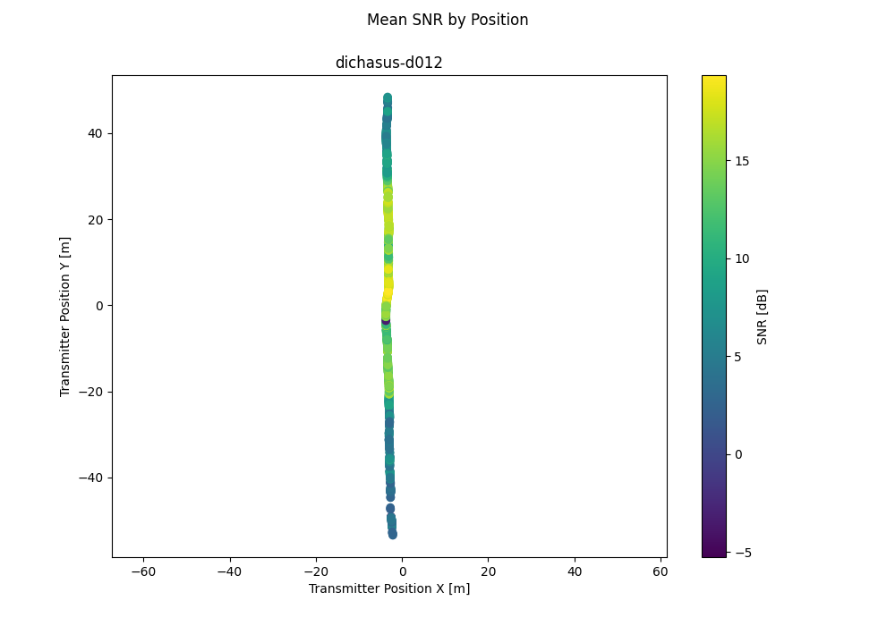
Position-Tagged
Experiment Setup


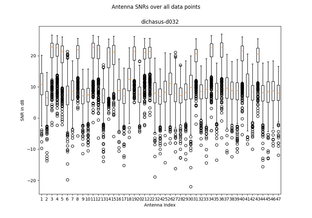
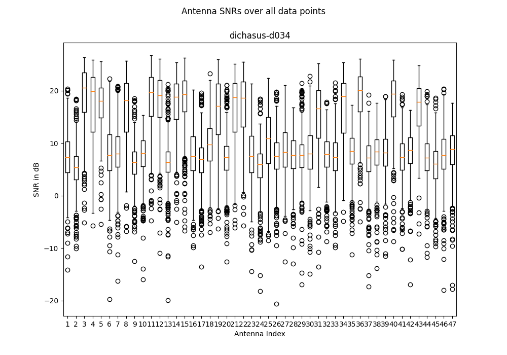
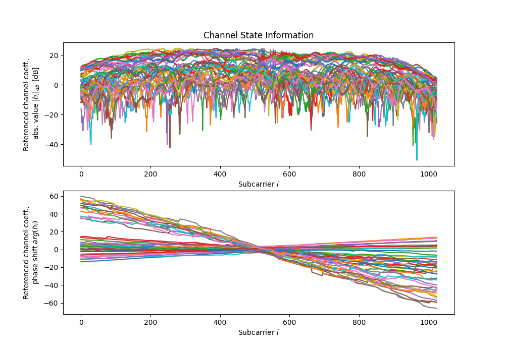
Data Analysis
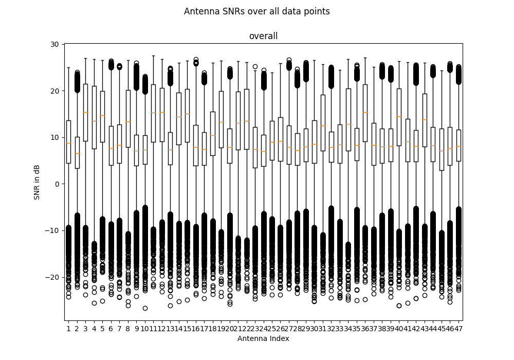
Antenna Configuration
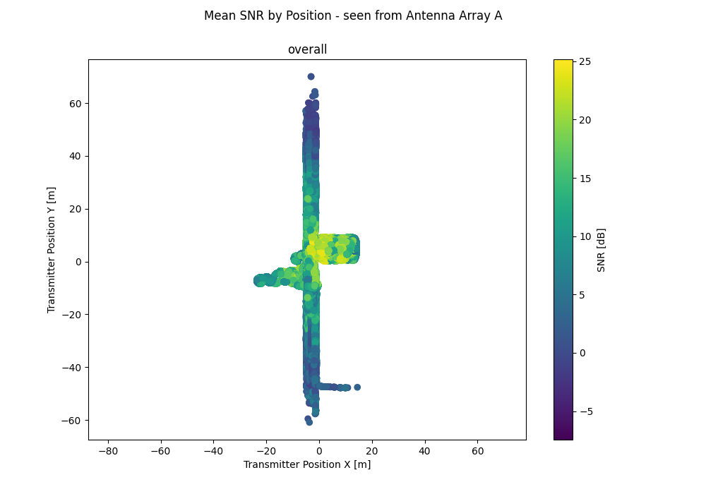
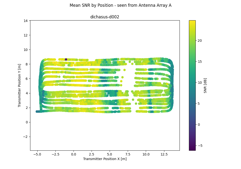
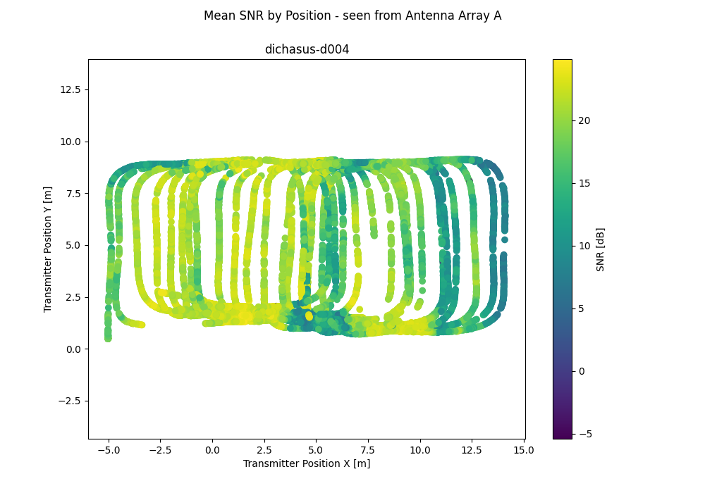
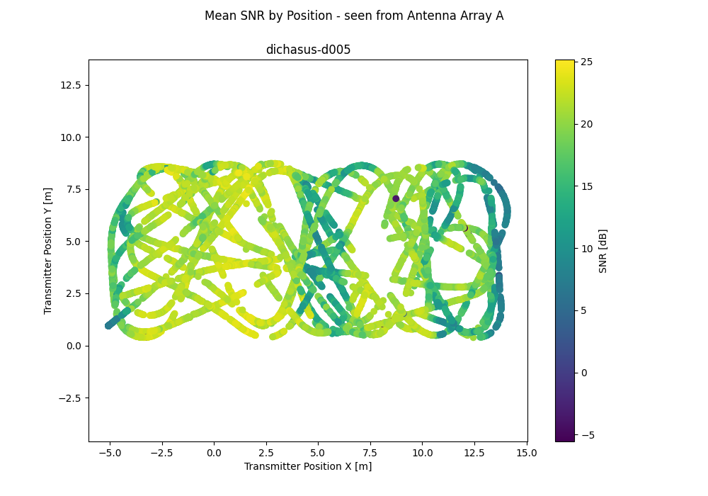
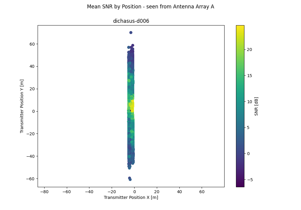
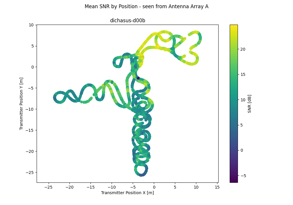
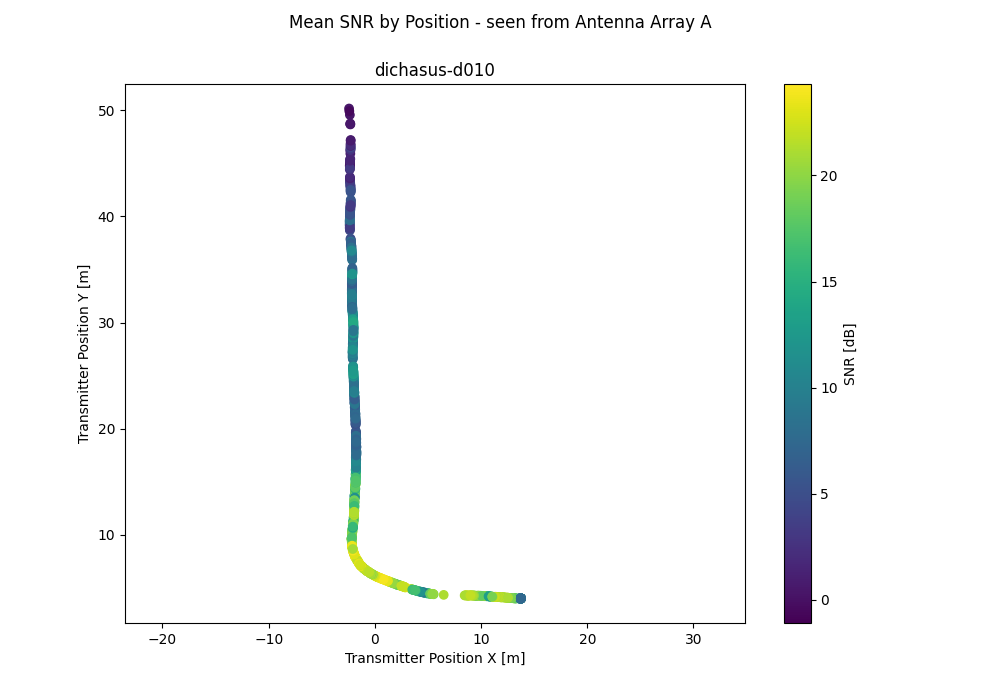
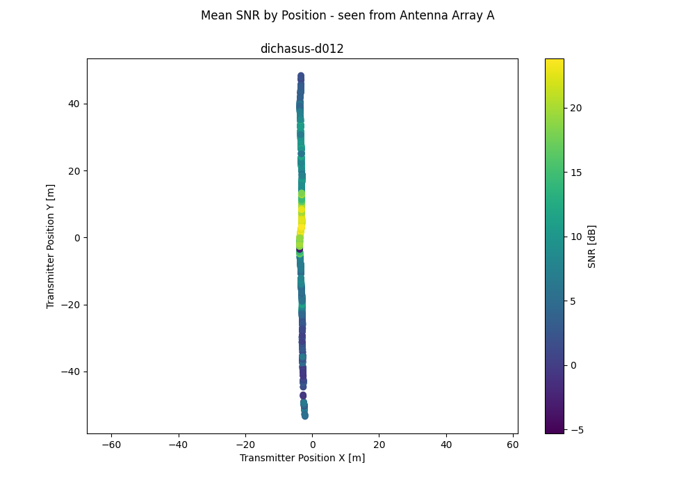
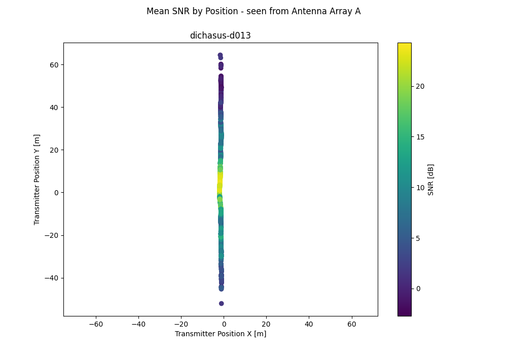
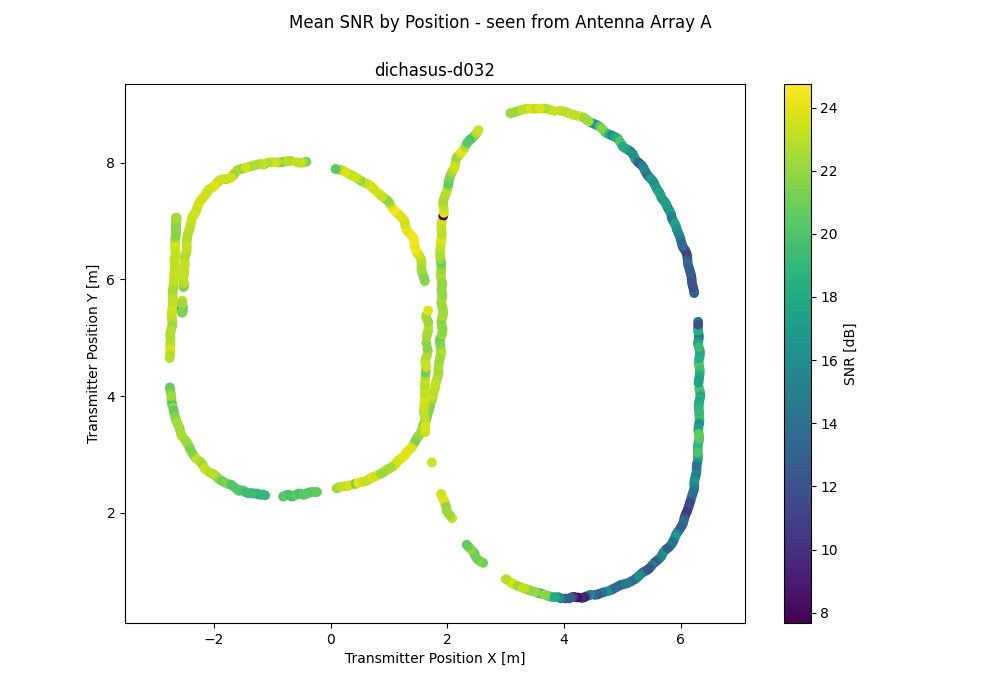
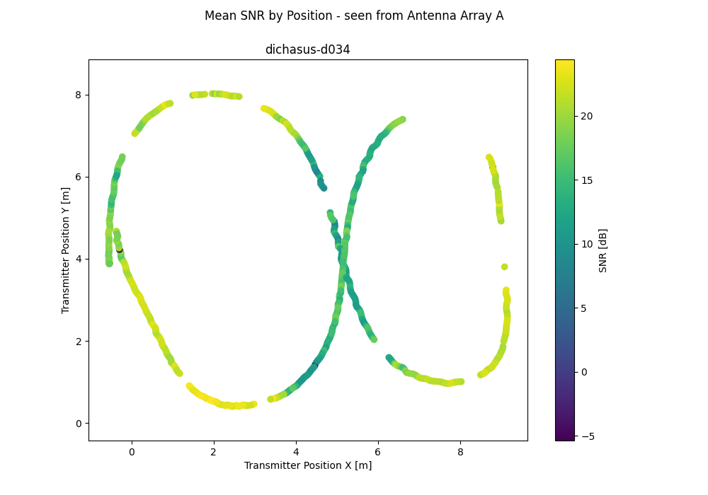
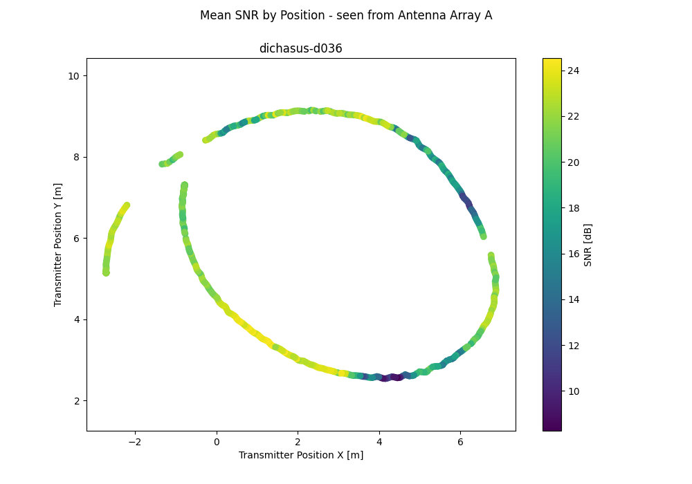
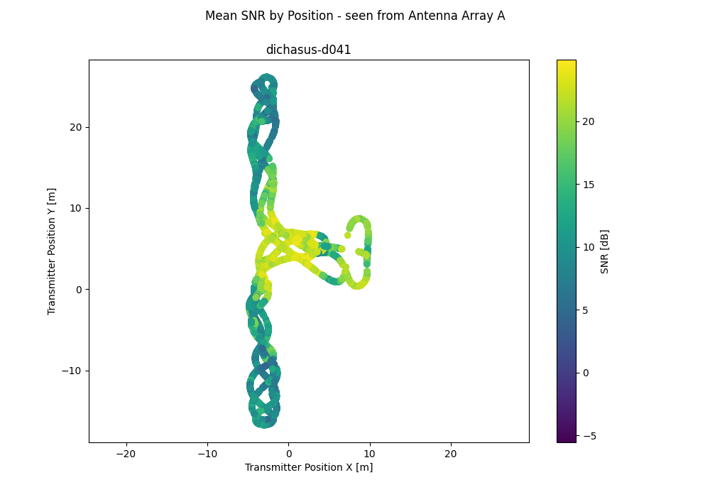
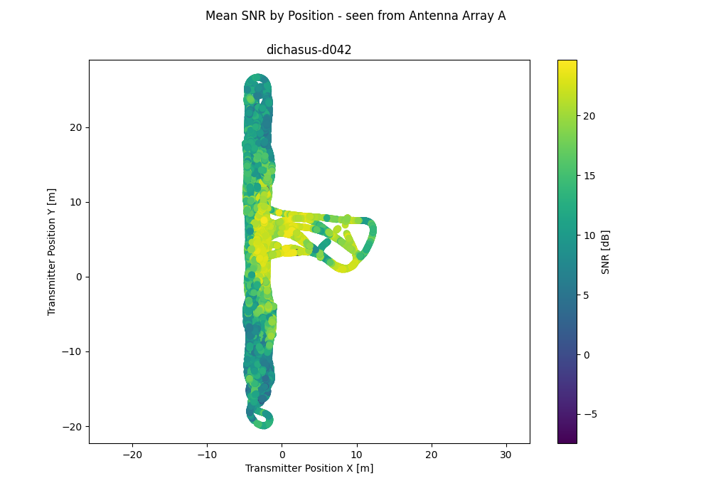
Antenna 1: Antenna Array A
| 4 | 13 | 39 | 14 | 2 | 35 | 10 | 11 |
| 42 | 33 | 30 | 18 | 7 | 20 | 3 | 21 |
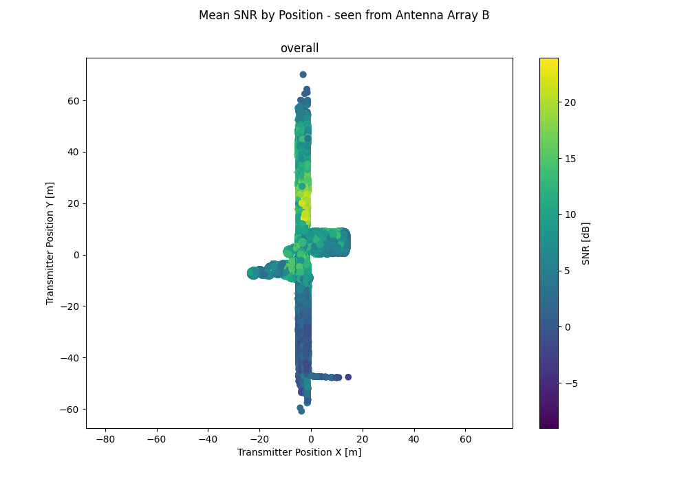
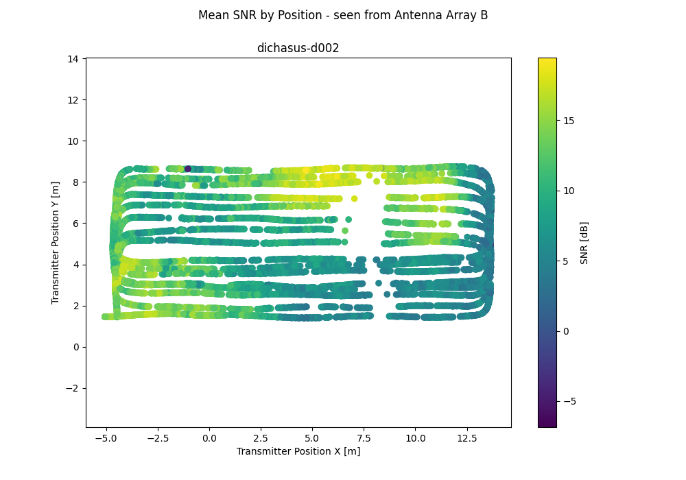
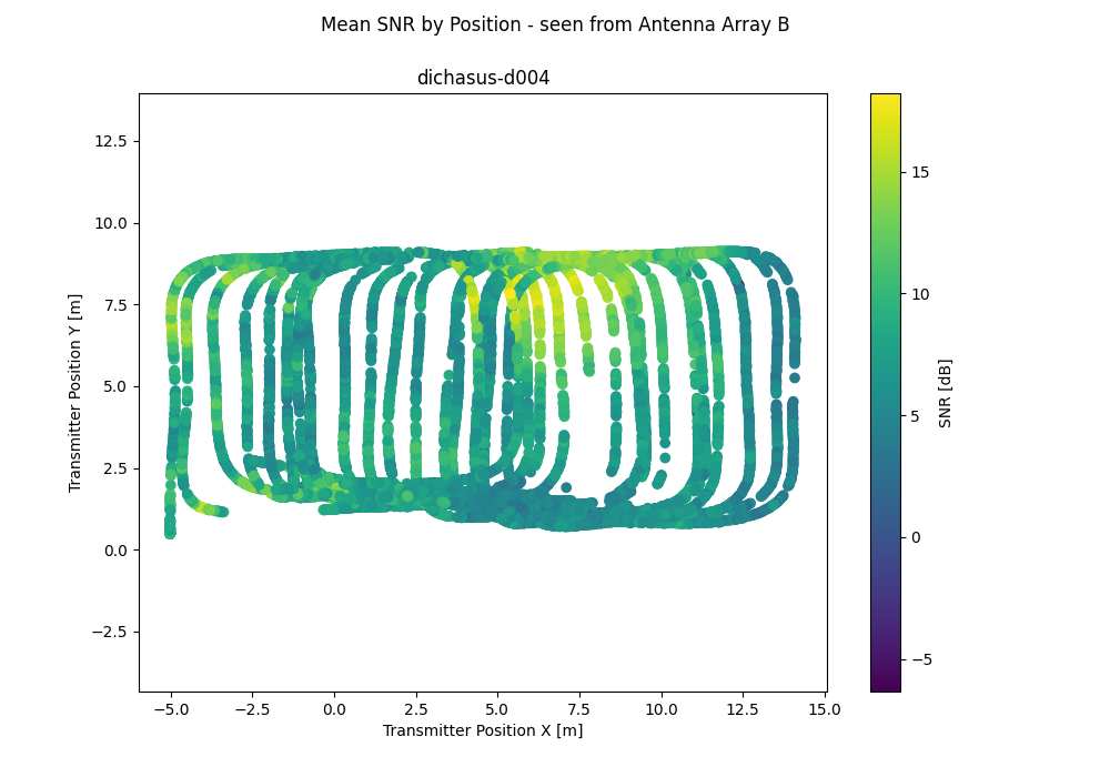
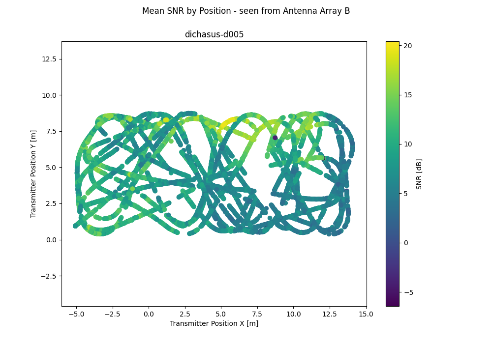
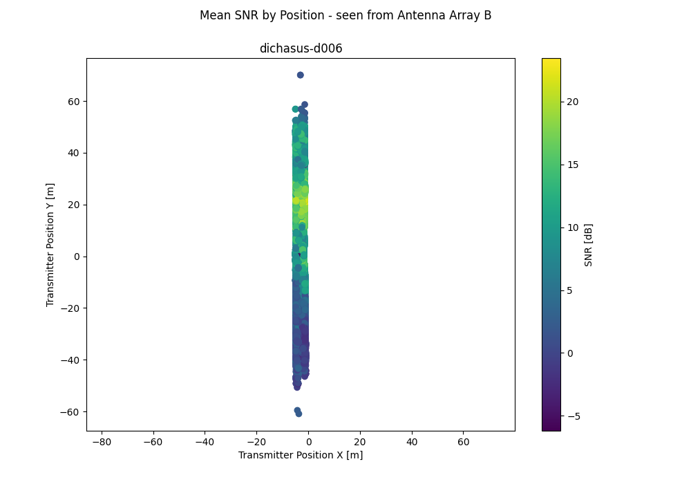
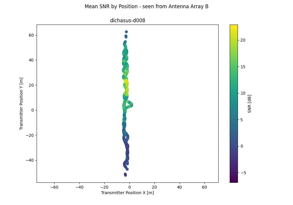
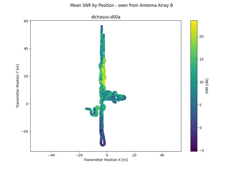
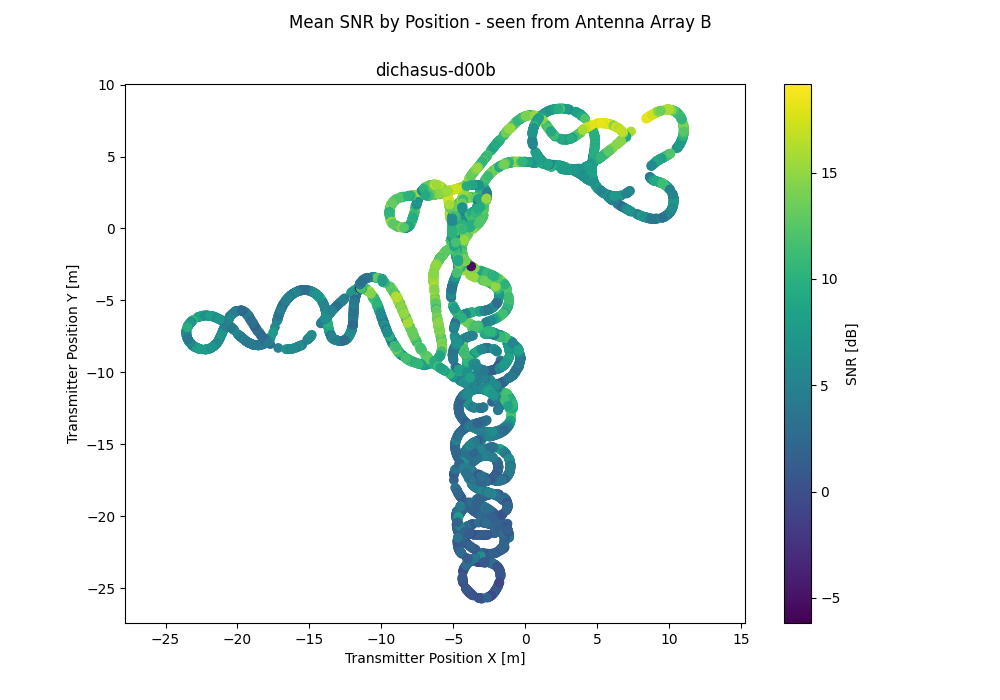
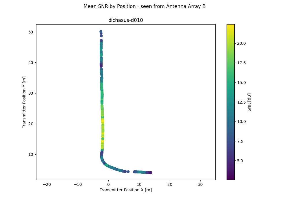
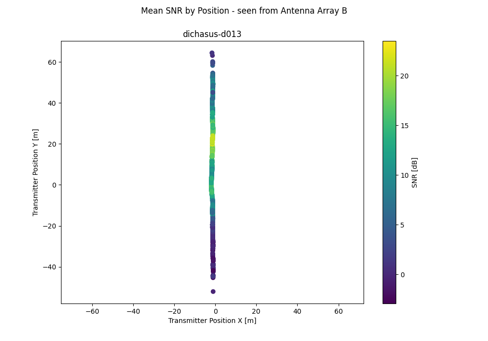
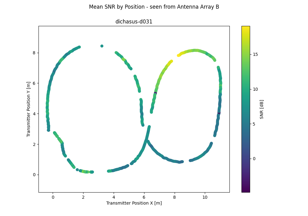
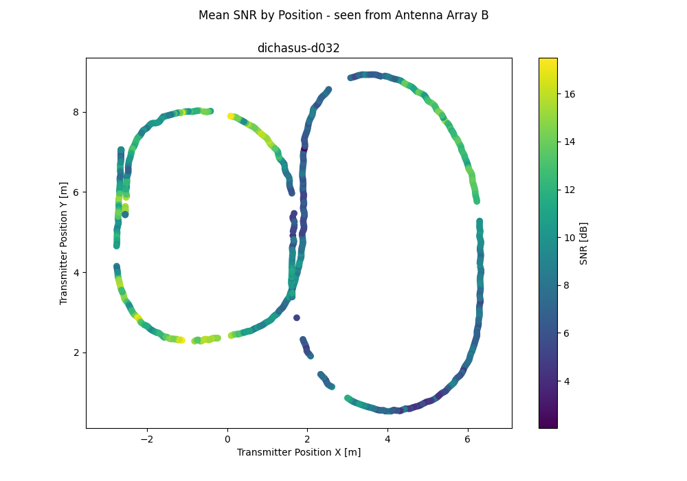
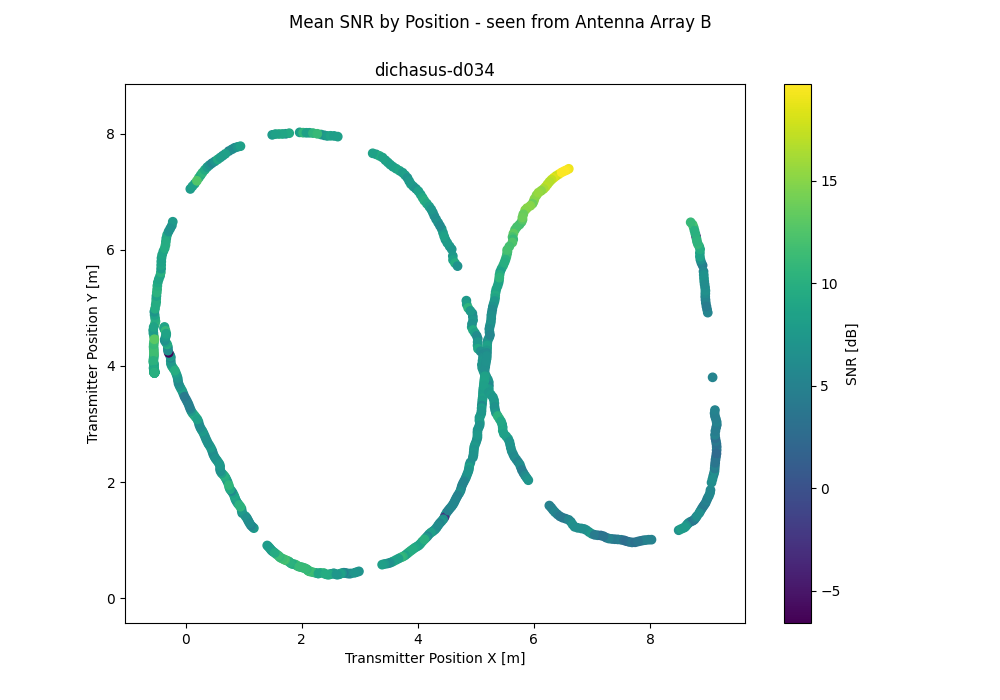
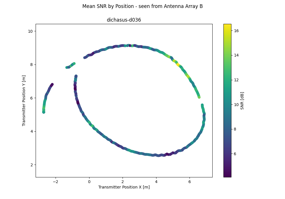
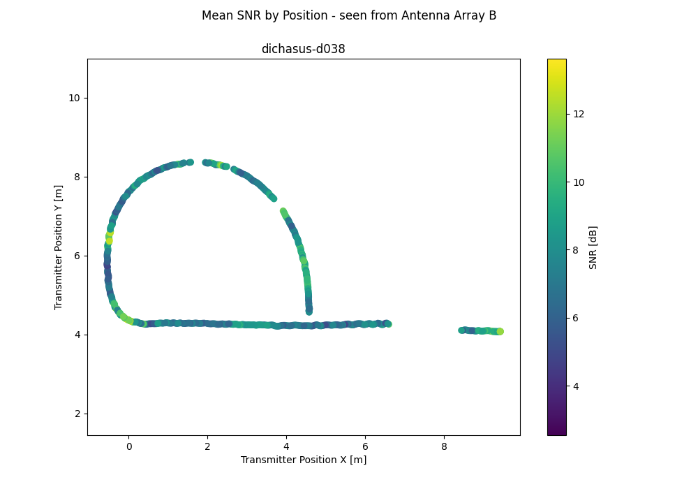
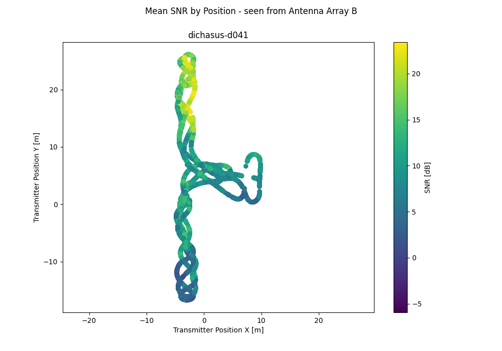
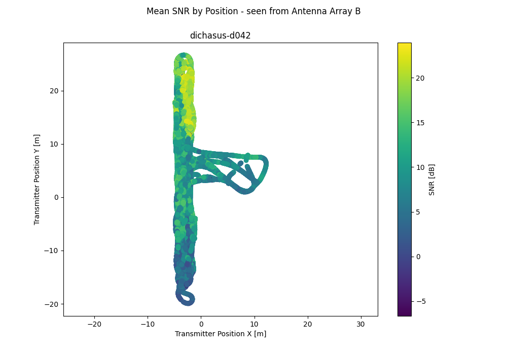
Antenna 2: Antenna Array B
| 32 | 40 | 44 | 36 | 25 | 0 | 17 | |
| 43 | 8 | 16 | 19 | 12 | 1 | 23 | 28 |
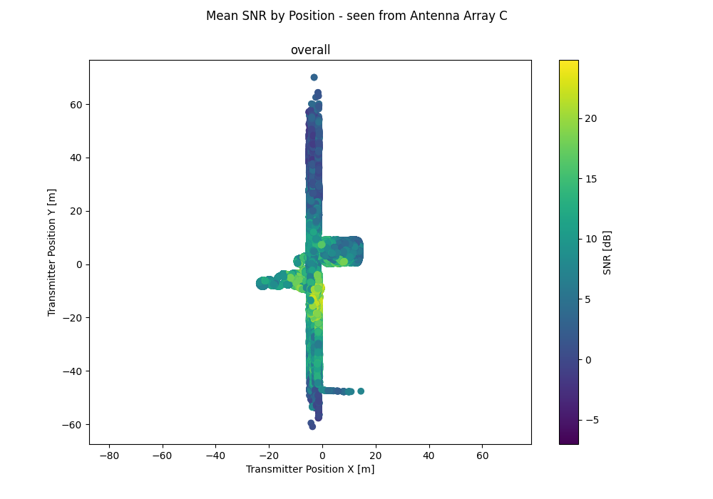
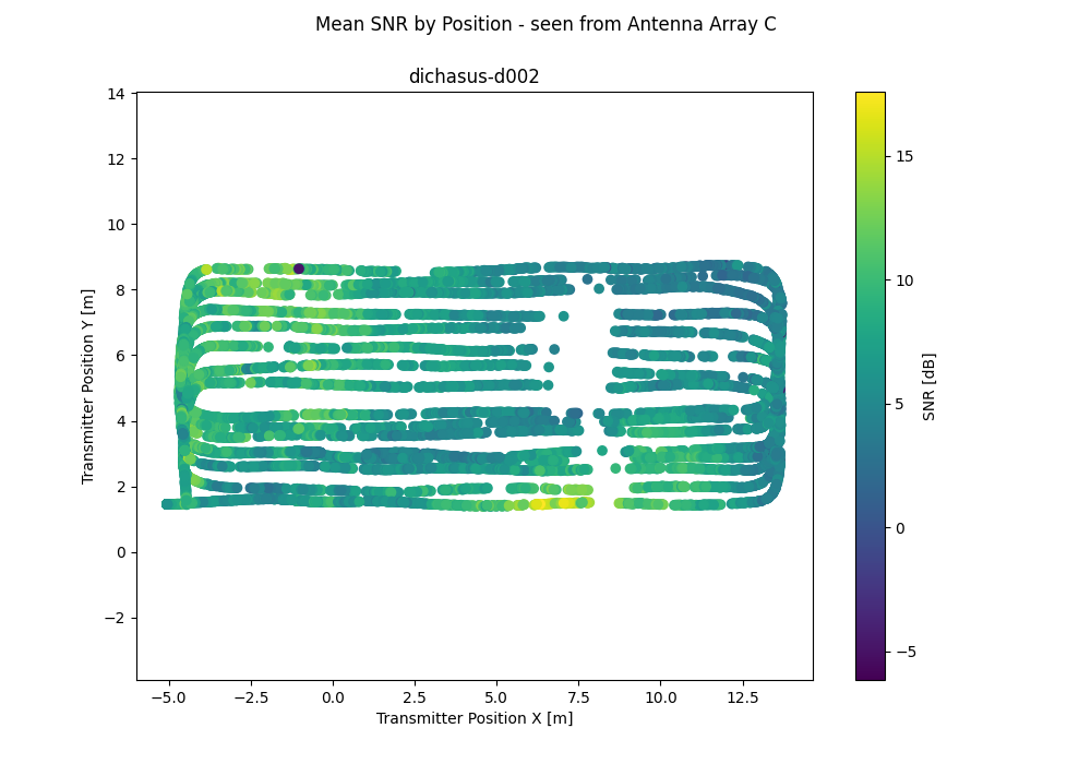
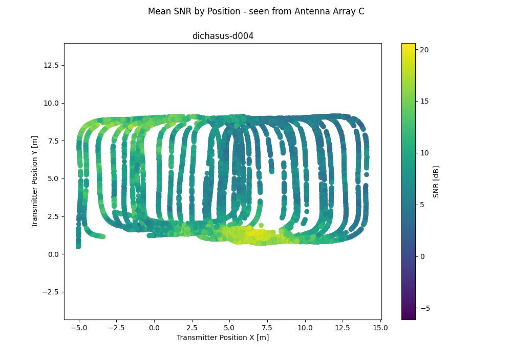
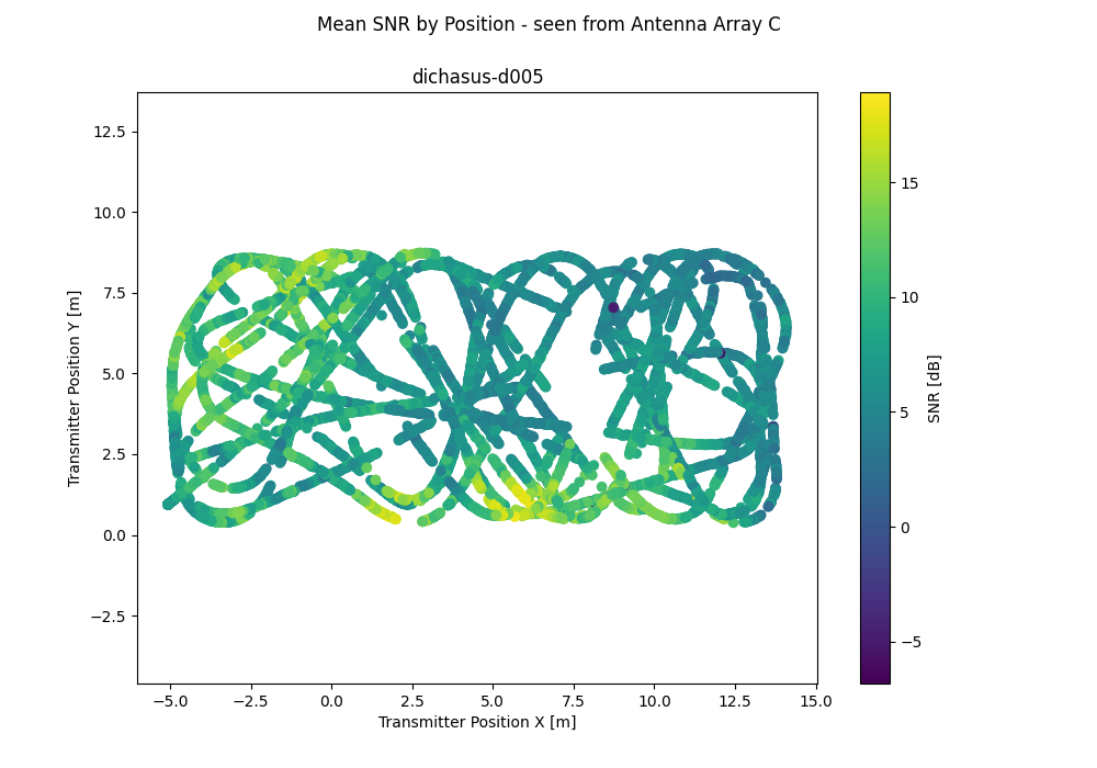
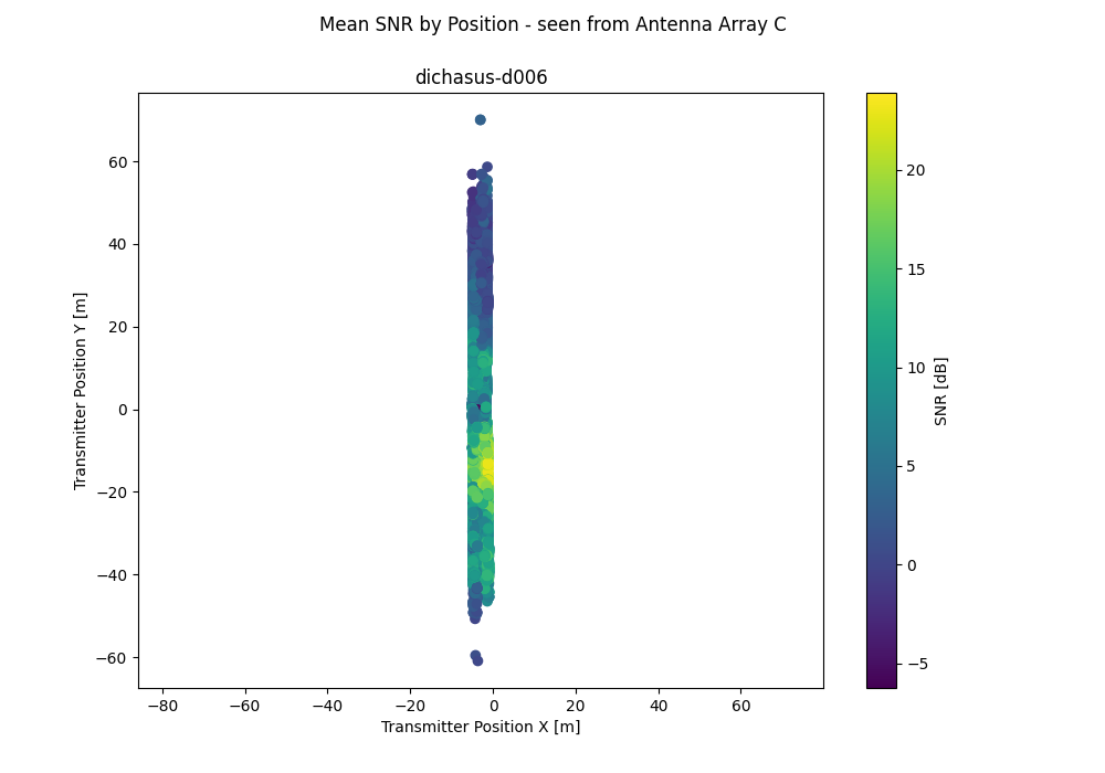
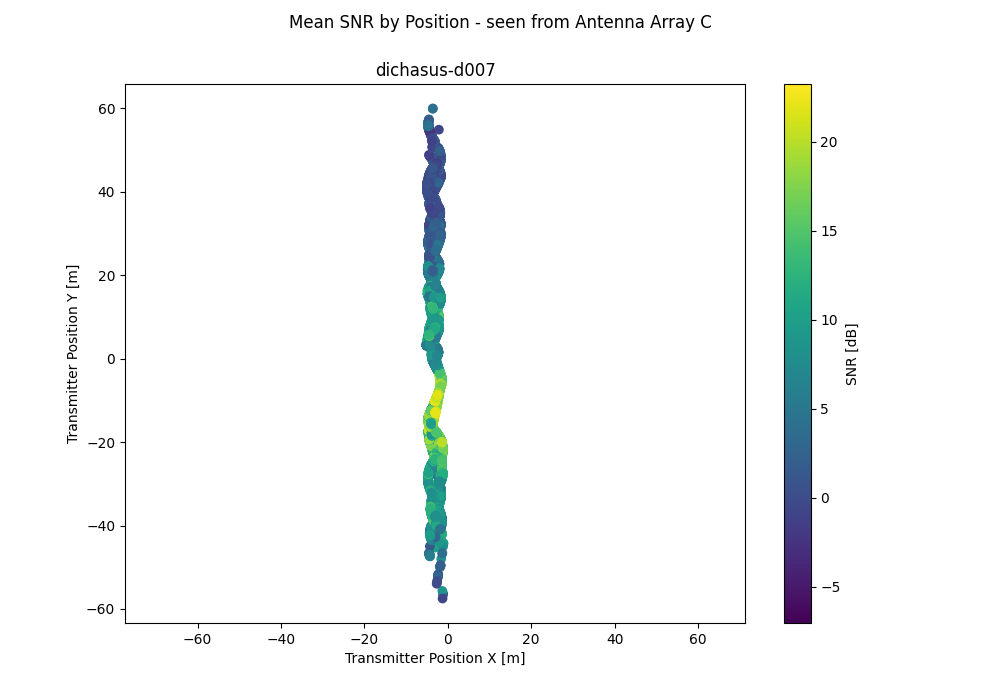
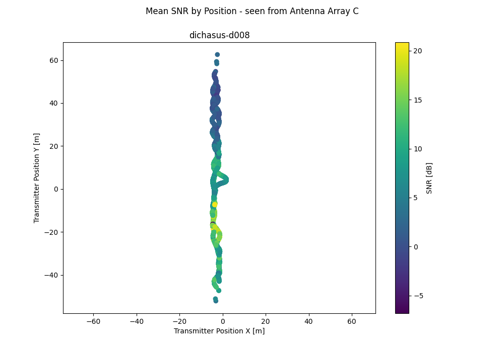
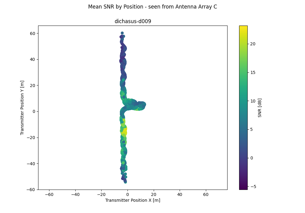
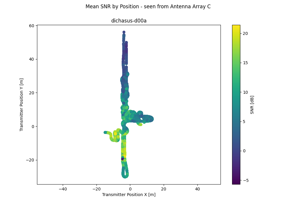
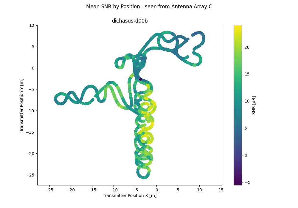
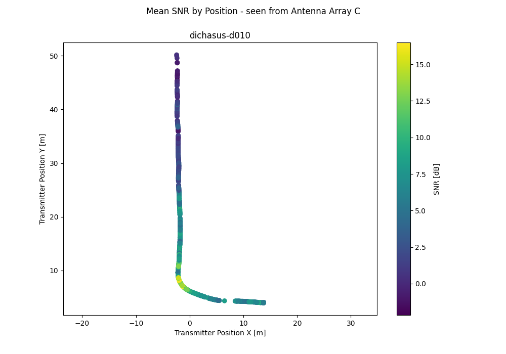
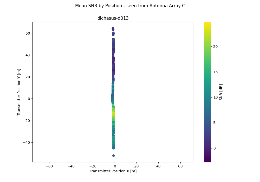
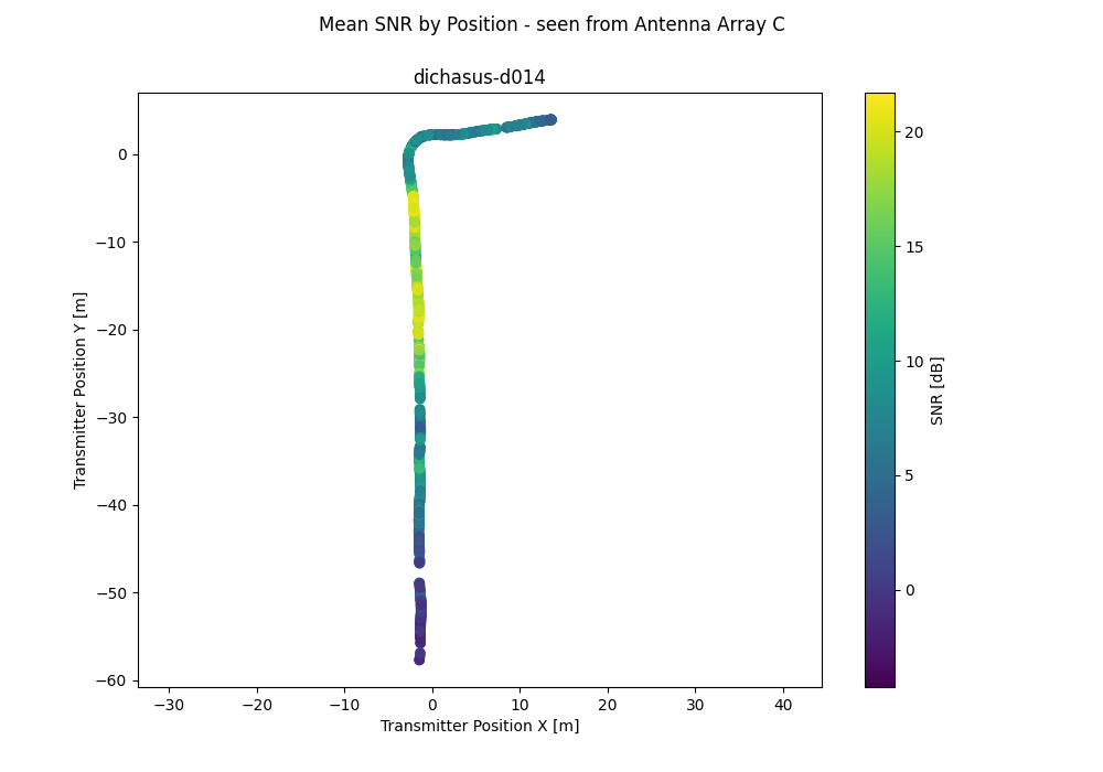
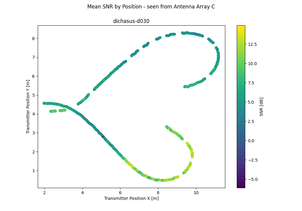
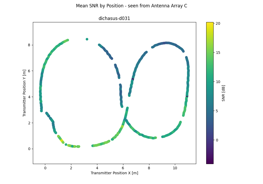
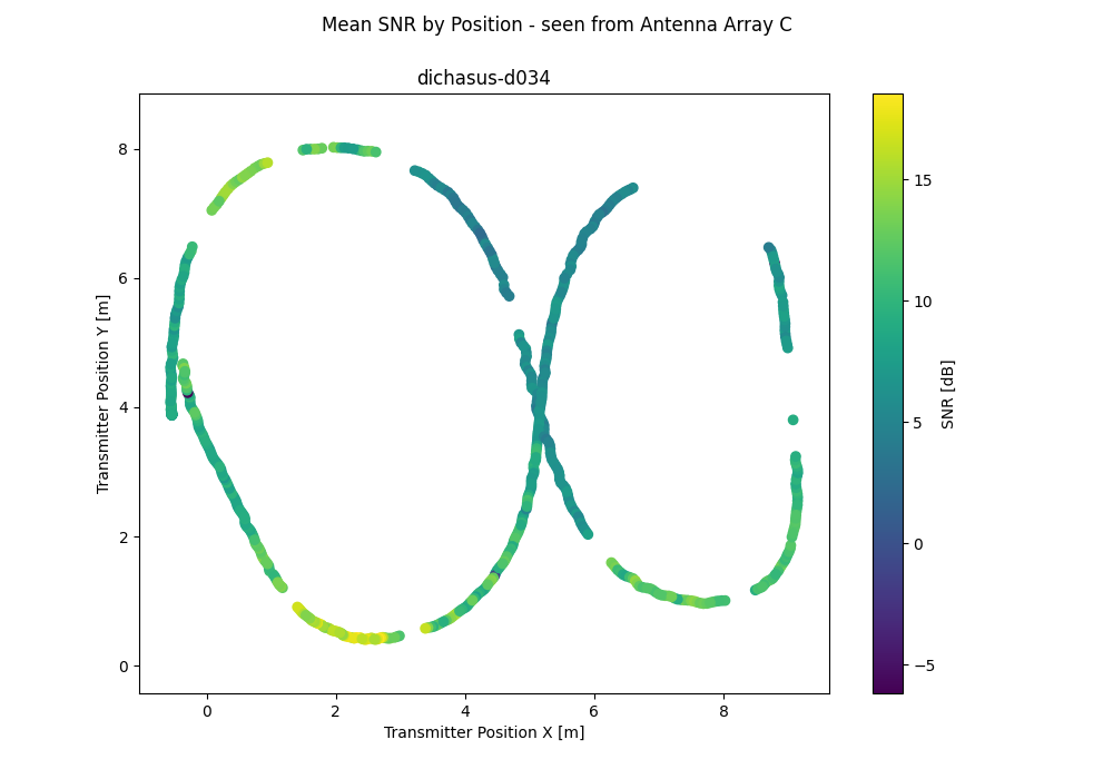
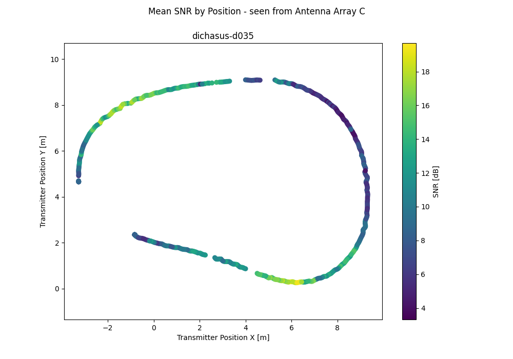
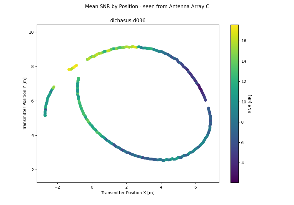
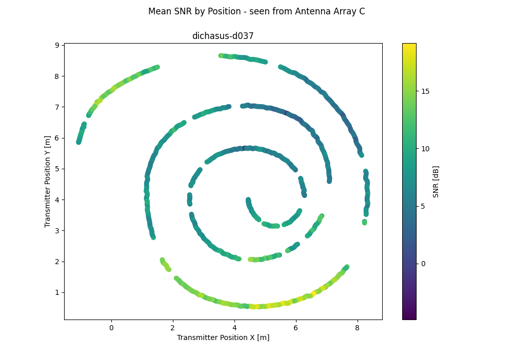
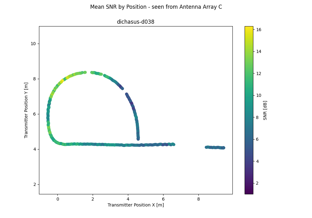
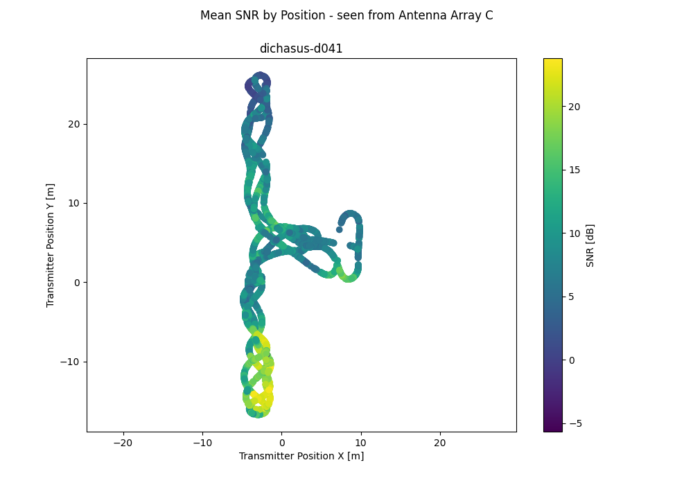
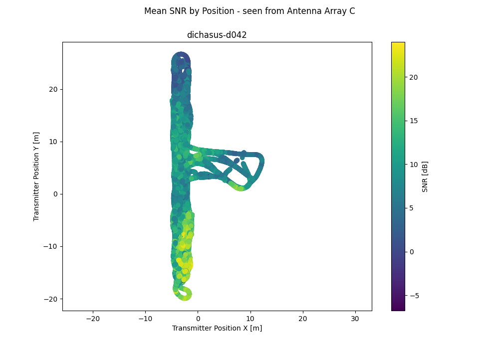
Antenna 3: Antenna Array C
| 24 | 5 | 26 | 22 | 15 | 45 | 29 | 6 |
| 46 | 9 | 41 | 27 | 34 | 37 | 31 | 38 |
Python: Import with TensorFlow
#!/usr/bin/env python3
import tensorflow as tf
raw_dataset = tf.data.TFRecordDataset(["tfrecords/dichasus-d002.tfrecords", "tfrecords/dichasus-d004.tfrecords", "tfrecords/dichasus-d005.tfrecords", "tfrecords/dichasus-d006.tfrecords", "tfrecords/dichasus-d007.tfrecords", "tfrecords/dichasus-d008.tfrecords", "tfrecords/dichasus-d009.tfrecords", "tfrecords/dichasus-d00a.tfrecords", "tfrecords/dichasus-d00b.tfrecords", "tfrecords/dichasus-d010.tfrecords", "tfrecords/dichasus-d011.tfrecords", "tfrecords/dichasus-d012.tfrecords", "tfrecords/dichasus-d013.tfrecords", "tfrecords/dichasus-d014.tfrecords", "tfrecords/dichasus-d020.tfrecords", "tfrecords/dichasus-d030.tfrecords", "tfrecords/dichasus-d031.tfrecords", "tfrecords/dichasus-d032.tfrecords", "tfrecords/dichasus-d033.tfrecords", "tfrecords/dichasus-d034.tfrecords", "tfrecords/dichasus-d035.tfrecords", "tfrecords/dichasus-d036.tfrecords", "tfrecords/dichasus-d037.tfrecords", "tfrecords/dichasus-d038.tfrecords", "tfrecords/dichasus-d041.tfrecords", "tfrecords/dichasus-d042.tfrecords"])
feature_description = {
"cfo": tf.io.FixedLenFeature([], tf.string, default_value = ''),
"csi": tf.io.FixedLenFeature([], tf.string, default_value = ''),
"gt-interp-age-tachy": tf.io.FixedLenFeature([], tf.float32, default_value = 0),
"pos-tachy": tf.io.FixedLenFeature([], tf.string, default_value = ''),
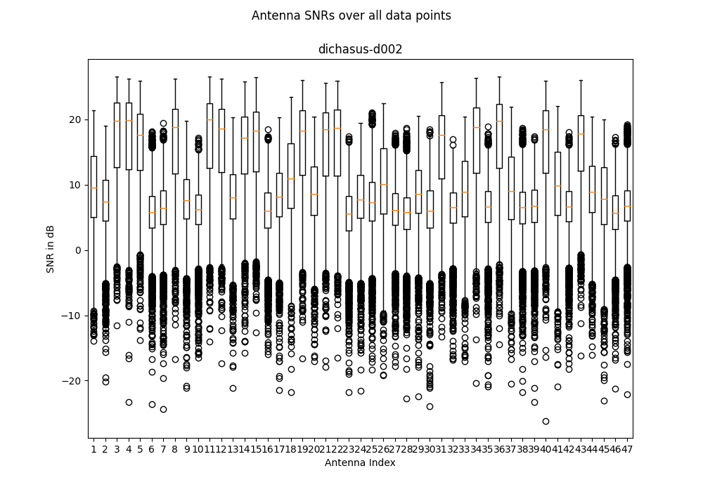
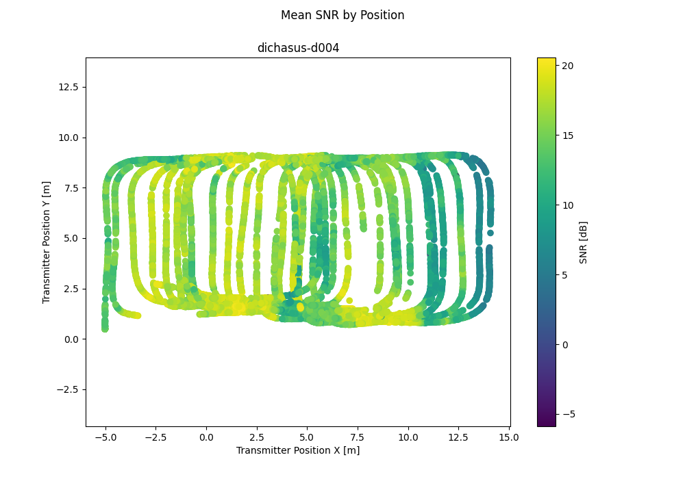
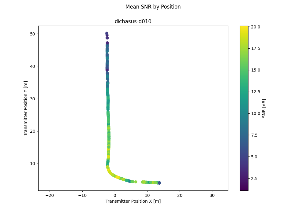
"snr": tf.io.FixedLenFeature([], tf.string, default_value = ''),
"time": tf.io.FixedLenFeature([], tf.float32, default_value = 0),
}
def record_parse_function(proto):
record = tf.io.parse_single_example(proto, feature_description)
# Measured carrier frequency offset between MOBTX and each receive antenna.
cfo = tf.ensure_shape(tf.io.parse_tensor(record["cfo"], out_type = tf.float32), (47))
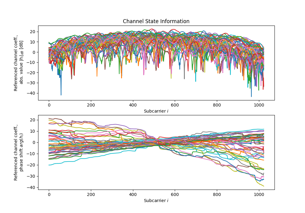
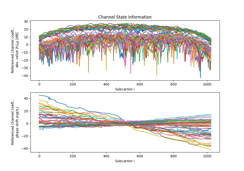
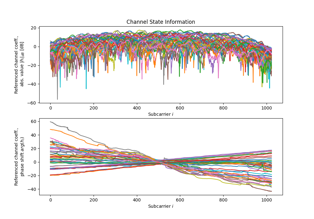
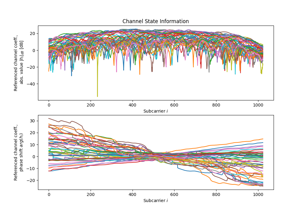
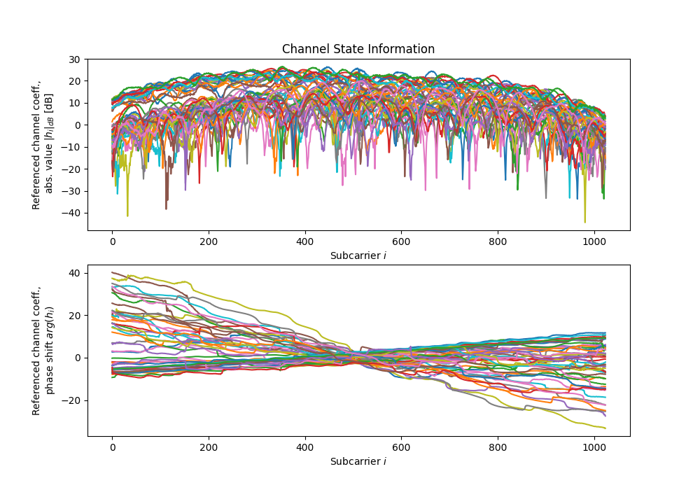
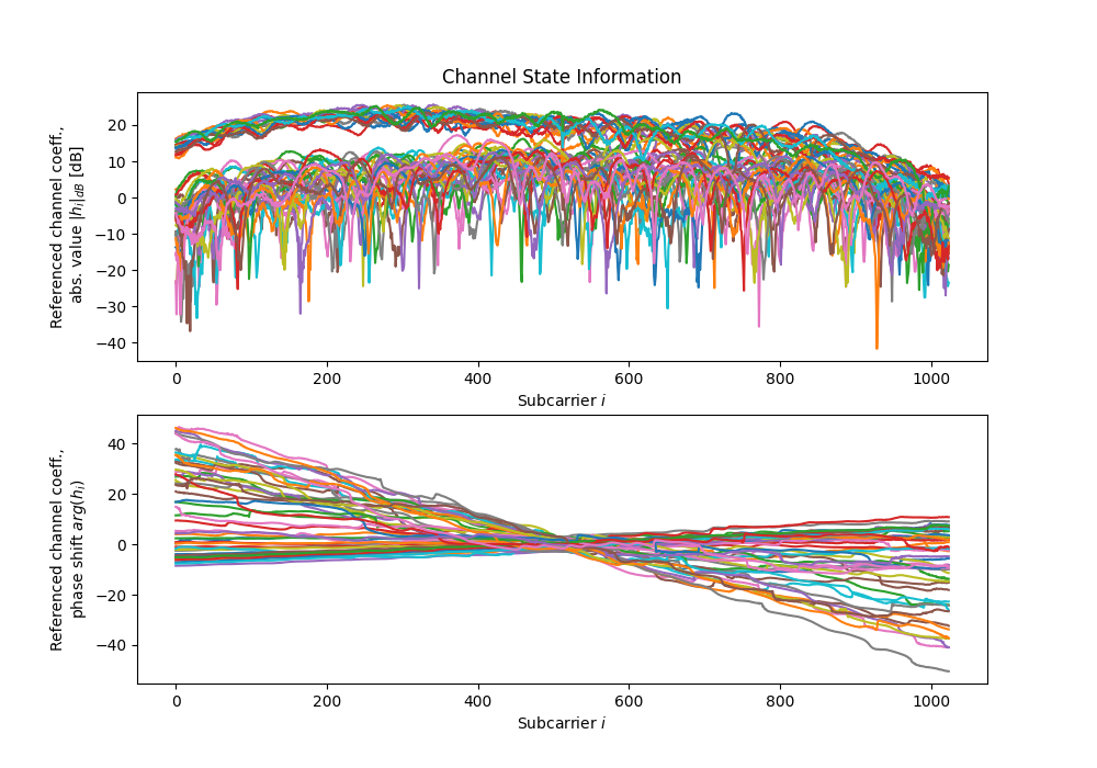
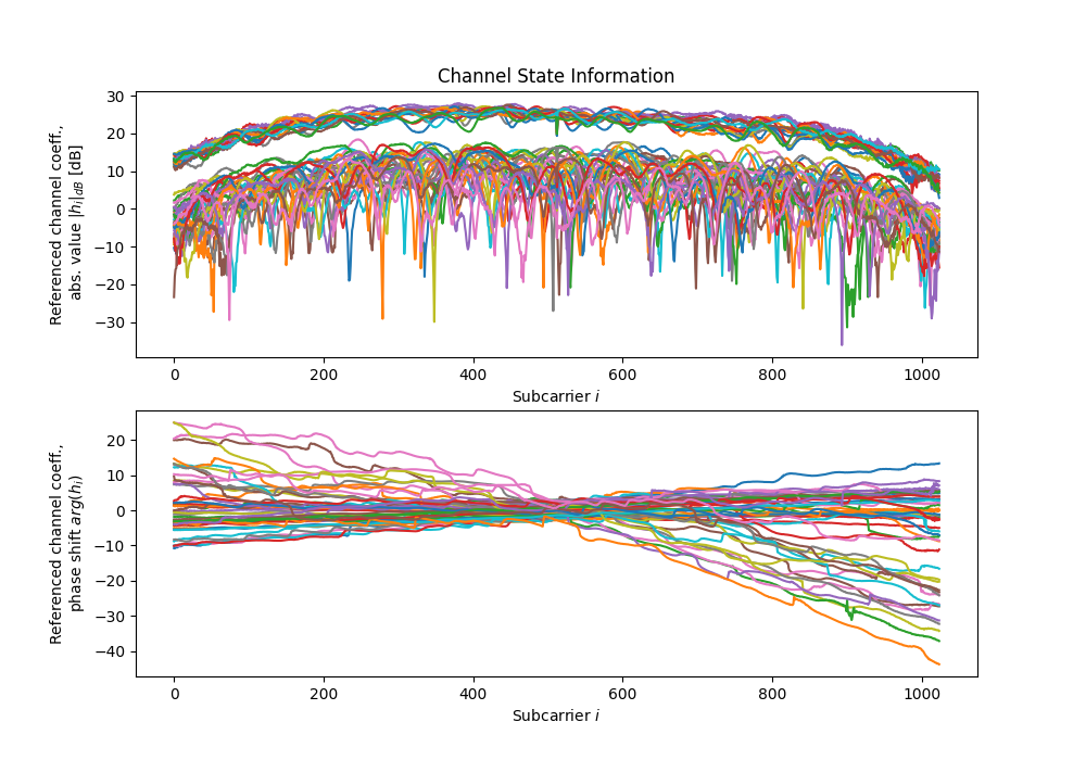
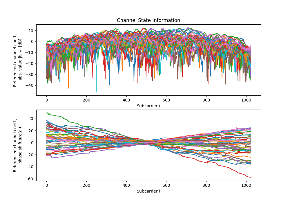
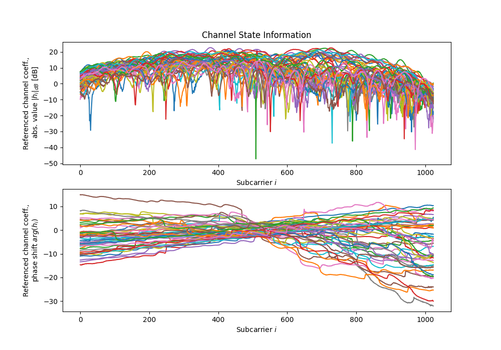
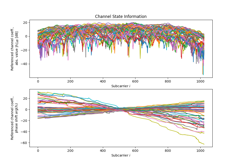
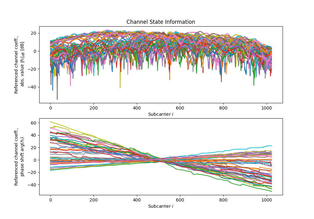
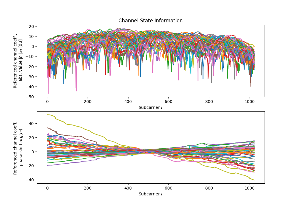
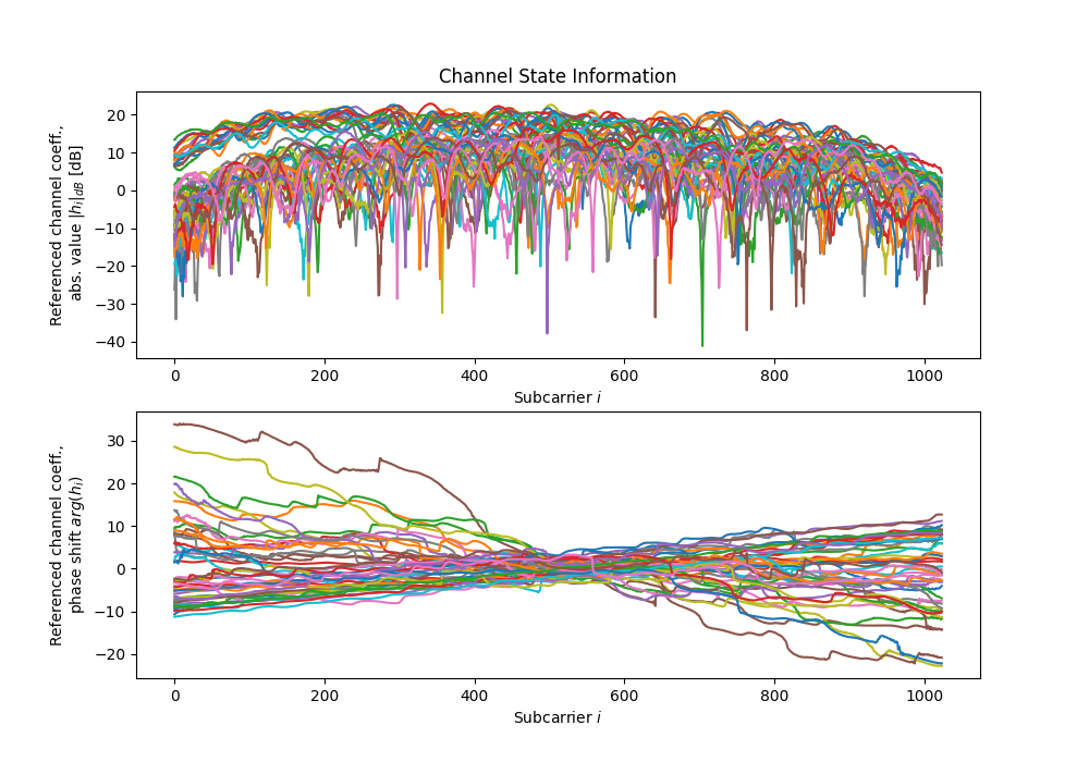
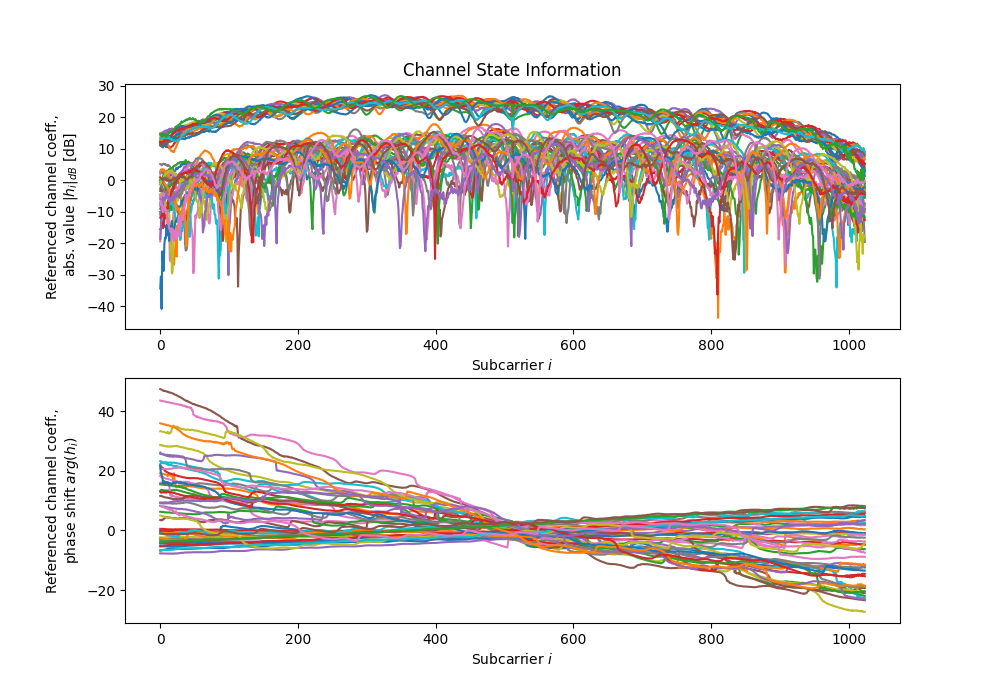
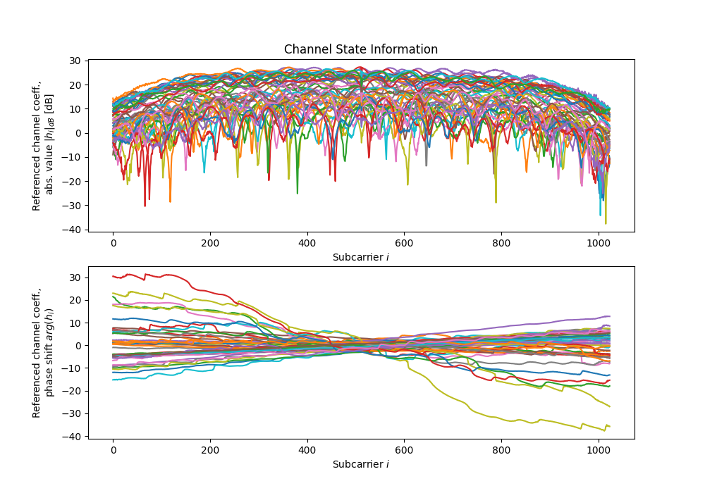
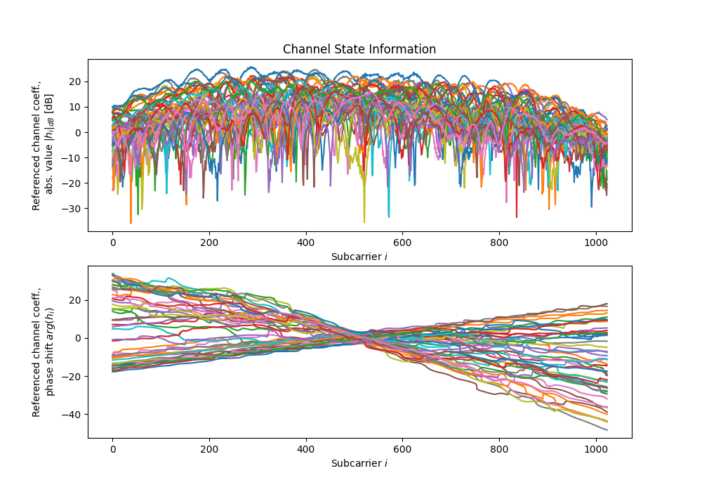
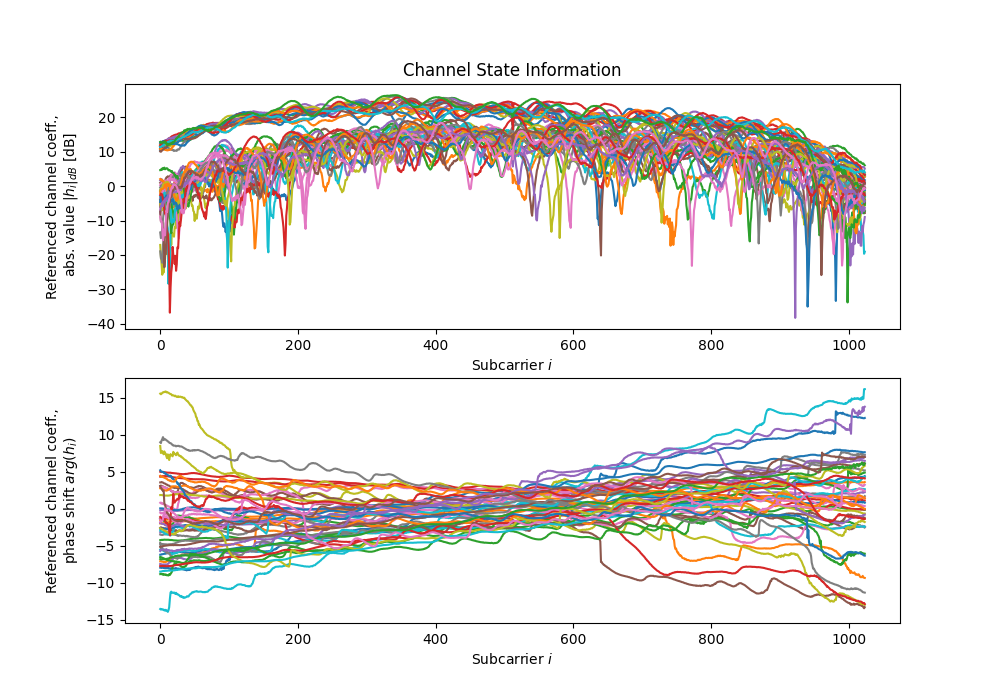
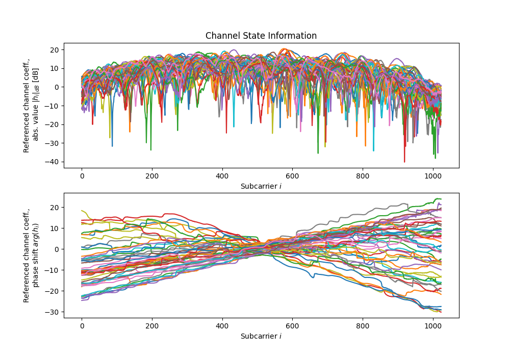
# Channel coefficients for all antennas, over all subcarriers, real and imaginary parts
csi = tf.ensure_shape(tf.io.parse_tensor(record["csi"], out_type = tf.float32), (47, 1024, 2))
# Time in seconds to closest known tachymeter position. Indicates quality of linear interpolation.
gt_interp_age_tachy = tf.ensure_shape(record["gt-interp-age-tachy"], ())
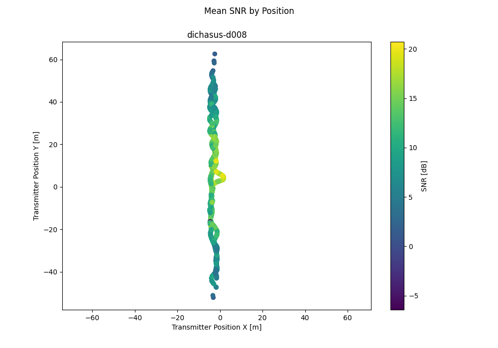
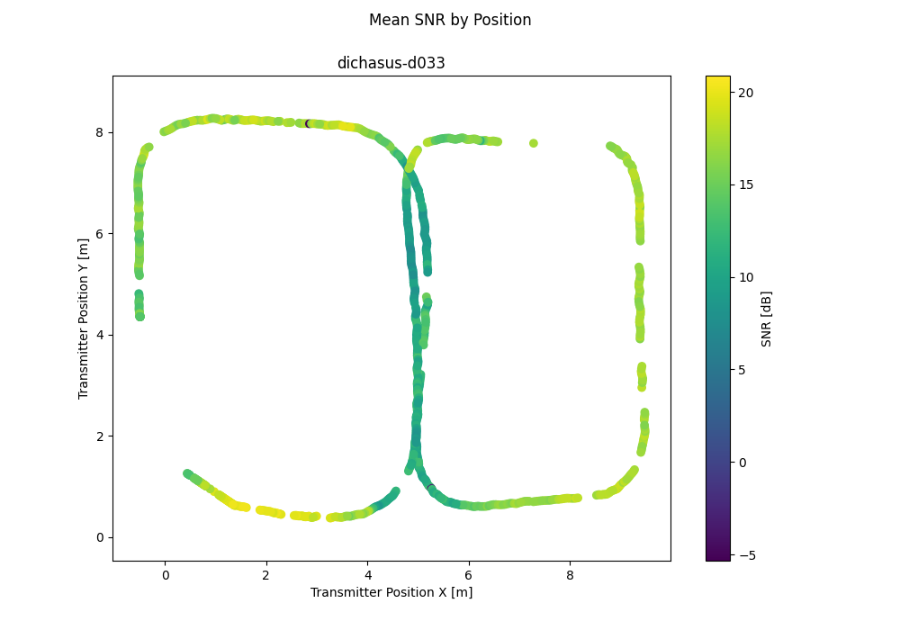
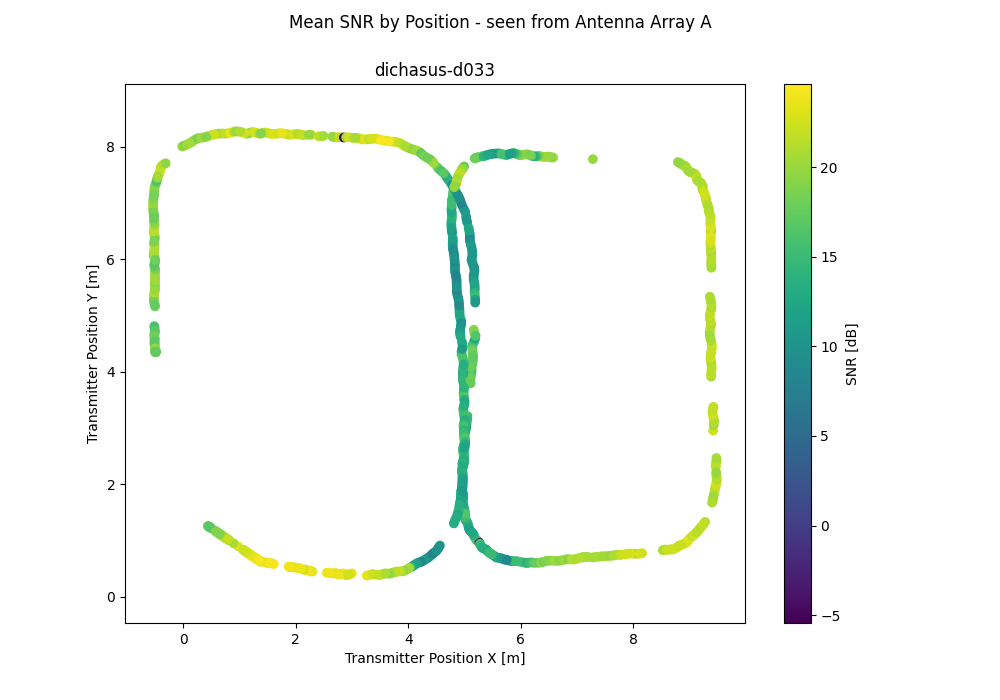
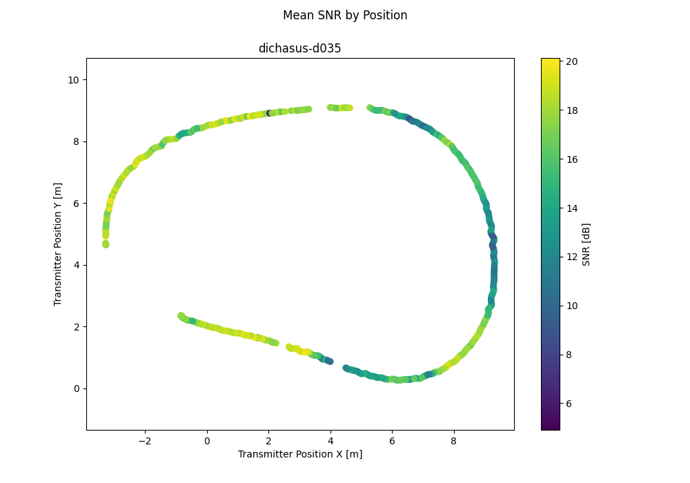
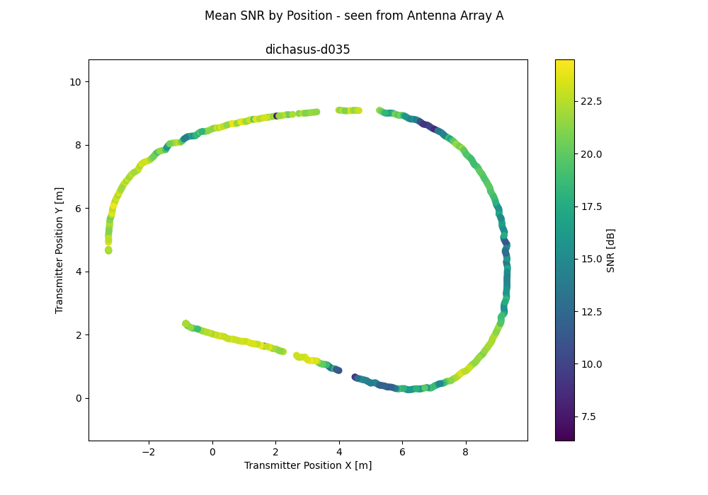
# Position of transmitter determined by a tachymeter pointed at a prism mounted on top of the antenna, in meters (X / Y / Z coordinates)
pos_tachy = tf.ensure_shape(tf.io.parse_tensor(record["pos-tachy"], out_type = tf.float64), (3))
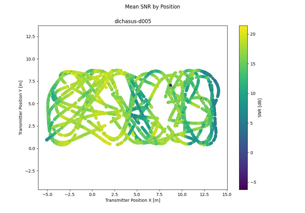
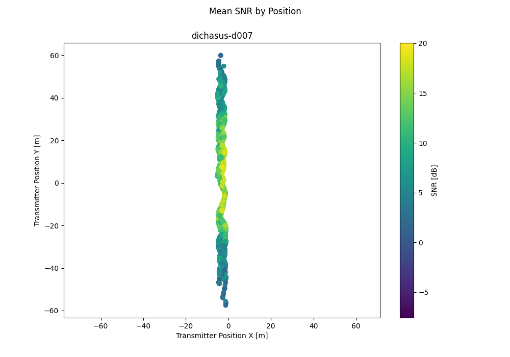
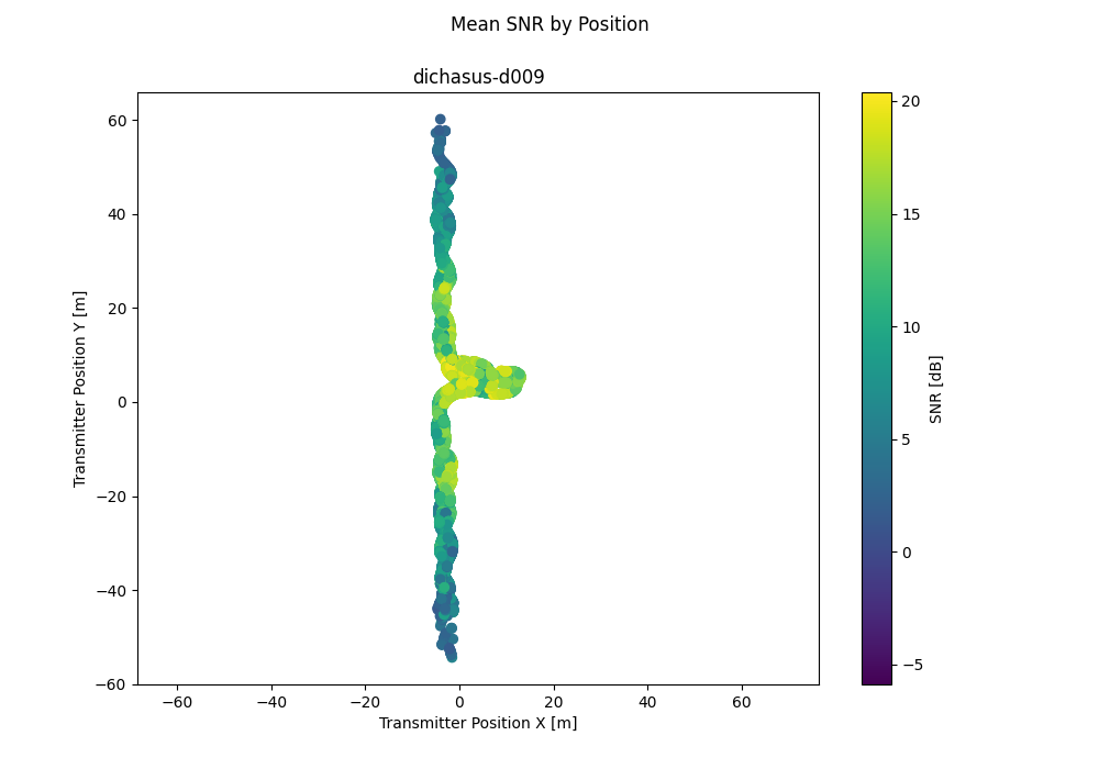
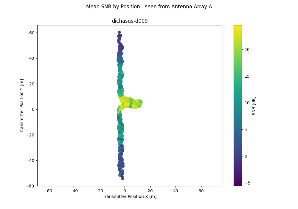
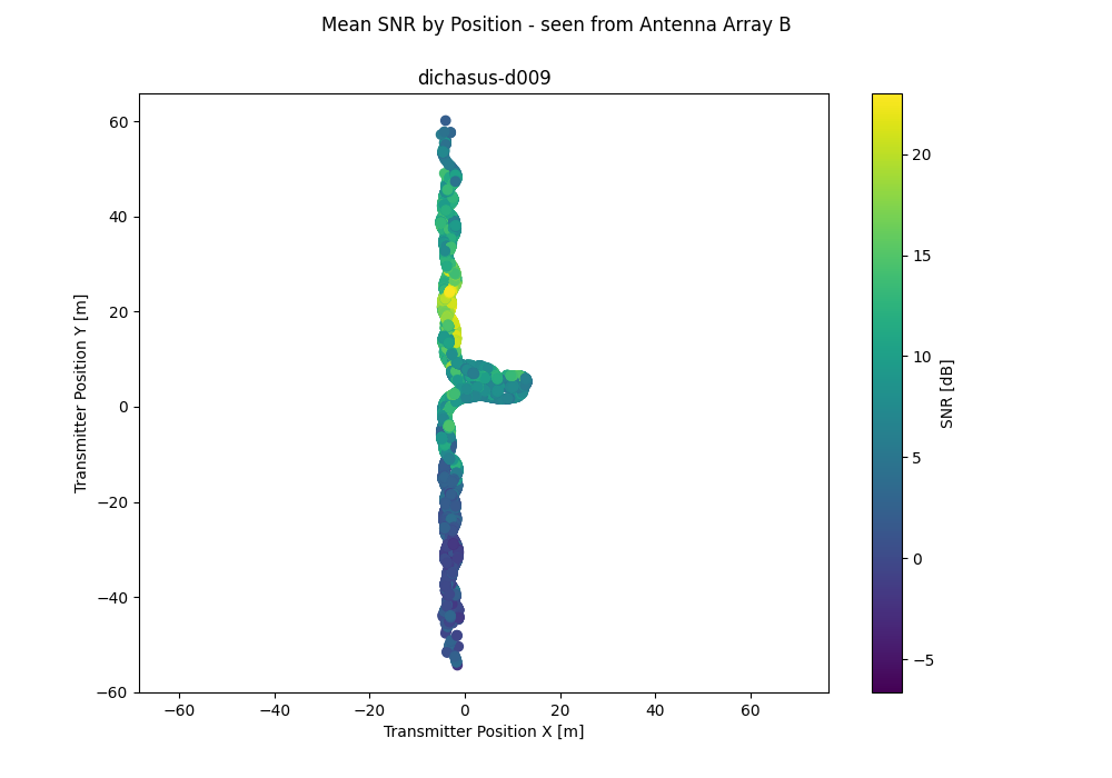
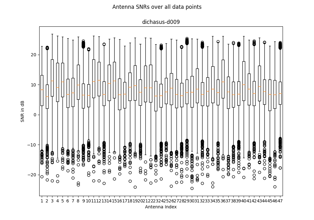
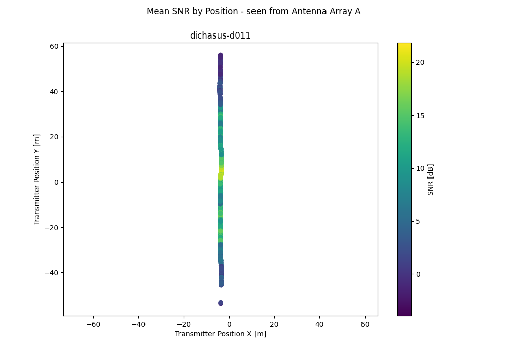
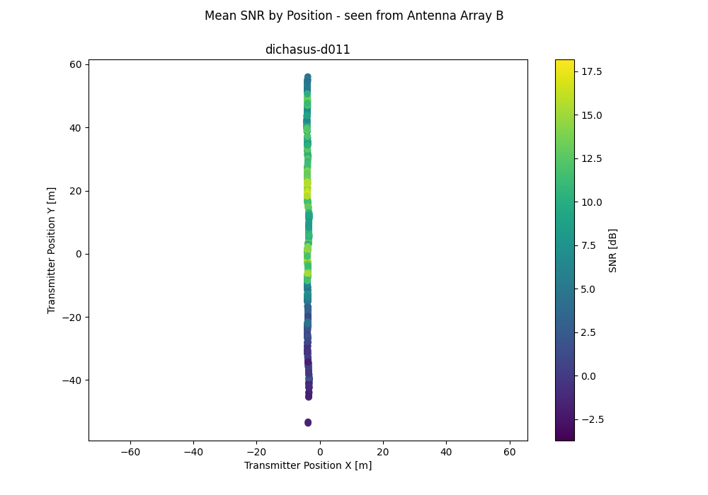
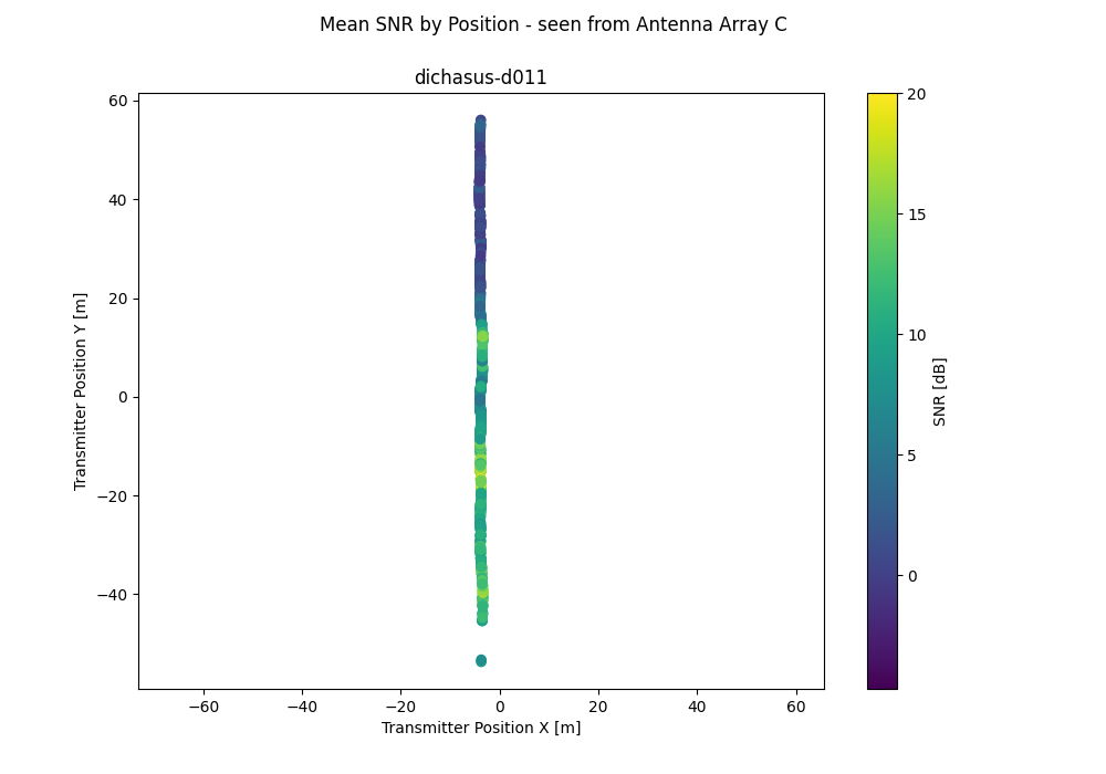
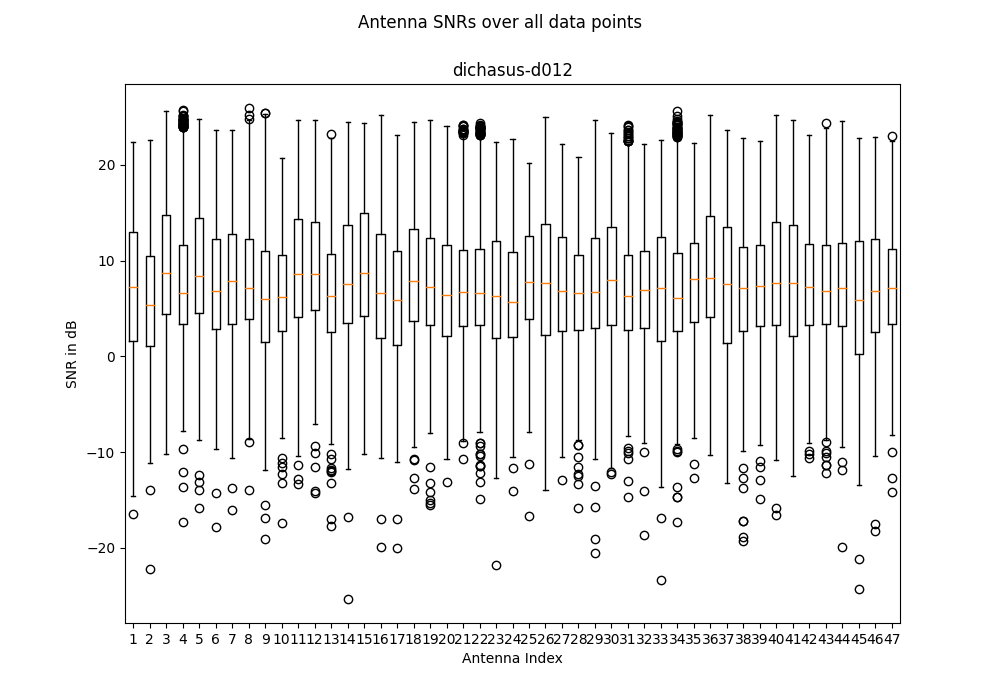
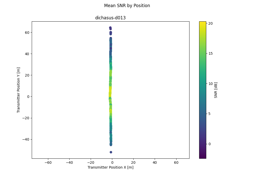
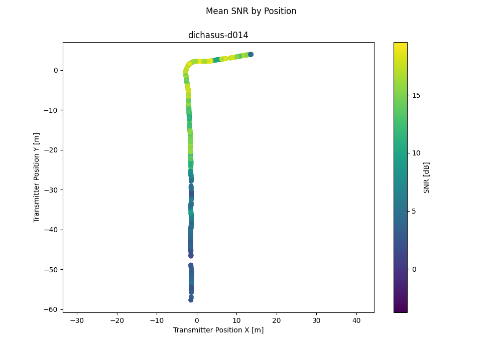
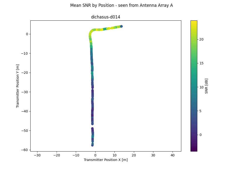
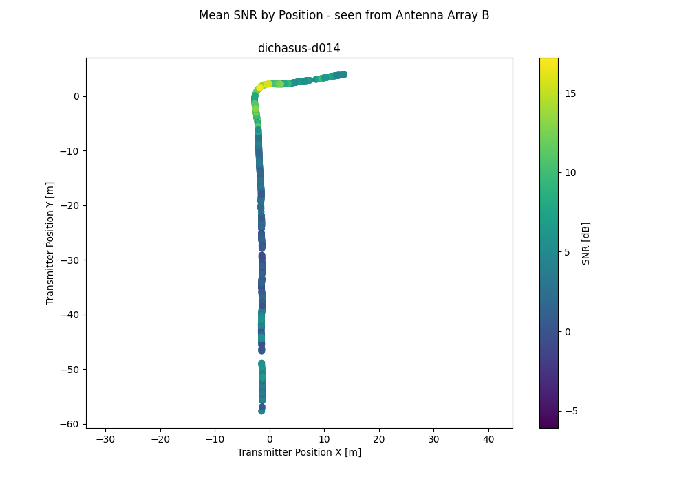
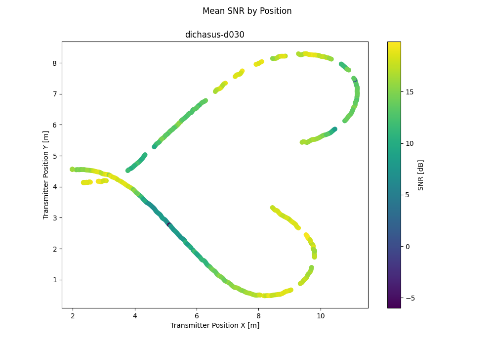
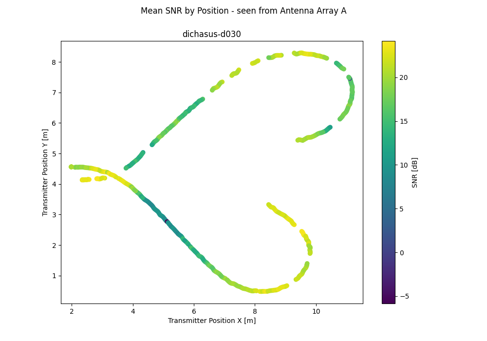
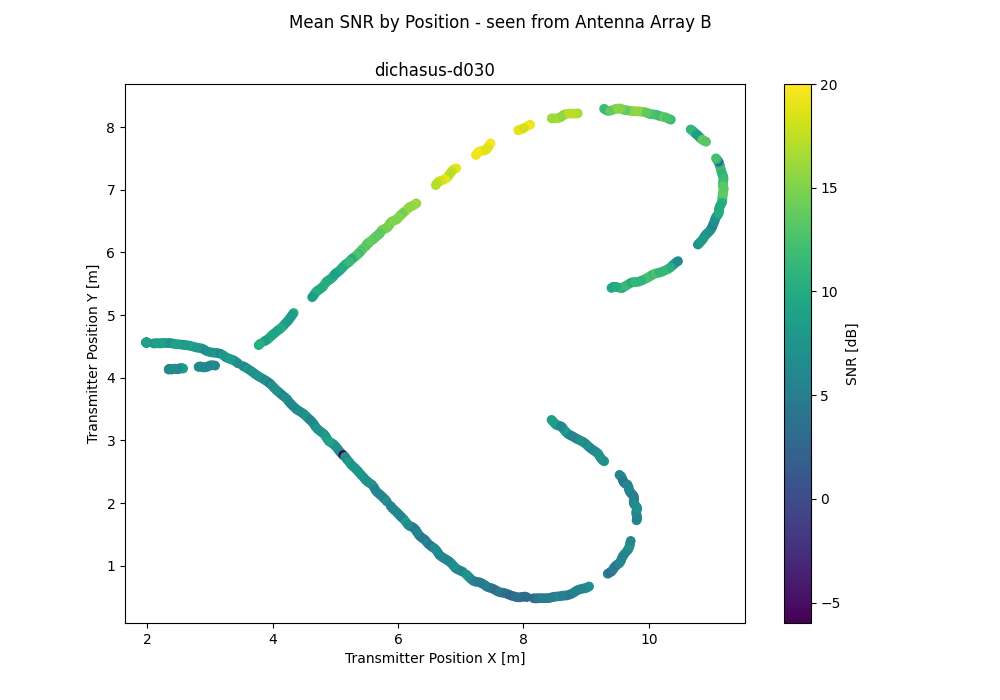
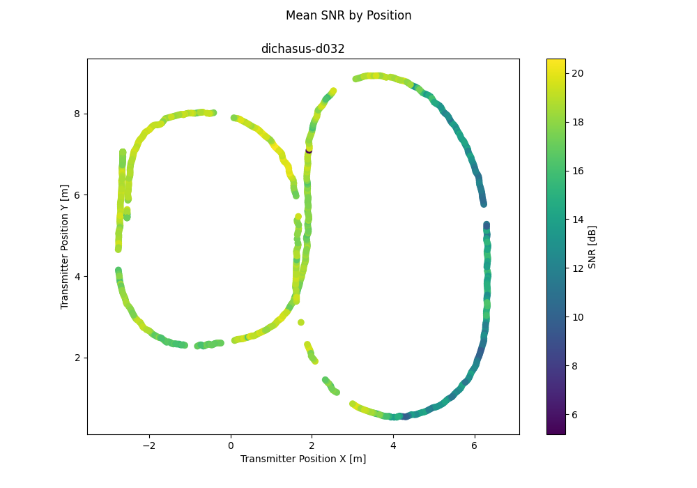
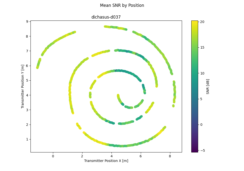
# Signal-to-Noise ratio estimates for all antennas
snr = tf.ensure_shape(tf.io.parse_tensor(record["snr"], out_type = tf.float32), (47))
# Timestamp since start of measurement campaign, in seconds
time = tf.ensure_shape(record["time"], ())
return cfo, csi, gt_interp_age_tachy, pos_tachy, snr, time
dataset = raw_dataset.map(record_parse_function, num_parallel_calls = tf.data.experimental.AUTOTUNE)
# Optional: Cache dataset in RAM for faster training
dataset = dataset.cache()Reference Channel Compensation
For this dataset, we are able to provide estimated antenna-specific carrier phase and sampling time offsets. These offsets occur due to the fact that the reference transmitter channel is not perfectly frequency-flat. To learn more about why these offsets occur and about their compensation, visit our offset calibration tutorial on this topic. Note that the estimates provided here are "best-effort" calculations. The phase and time offsets between antennas in the same array are usually very accurate, but for antennas that are spaced far apart, the results may be less precise. For this dataset, the reference transmitter channel seems to be somewhat unstable, i.e., phase and time offsets fluctuate over time. Therefore, we provide a file containing our phase and time offset estimates for each individual file in the dataset. You can download these estimates from the list of files below.How to Cite
Please refer to the home page for information on how to cite any of our datasets in your research. For this dataset in particular, you may use the following BibTeX:
@data{dataset-dichasus-dxxx-reduced,
	author    = {Euchner, Florian and Gauger, Marc},
	publisher = {DaRUS},
	title     = {{CSI Dataset dichasus-dxxx-reduced: Outdoor - Three arrays distributed along the facade (one antenna removed)}},
	doi       = {doi:10.18419/darus-3236},
	url       = {https://doi.org/doi:10.18419/darus-3236},
	year      = {2022}
}
Download
This dataset consists of 26 files. Descriptions of these files as well as download links are provided below.
dichasus-d002
dichasus-d004
dichasus-d005
dichasus-d006
dichasus-d007
dichasus-d008
dichasus-d009
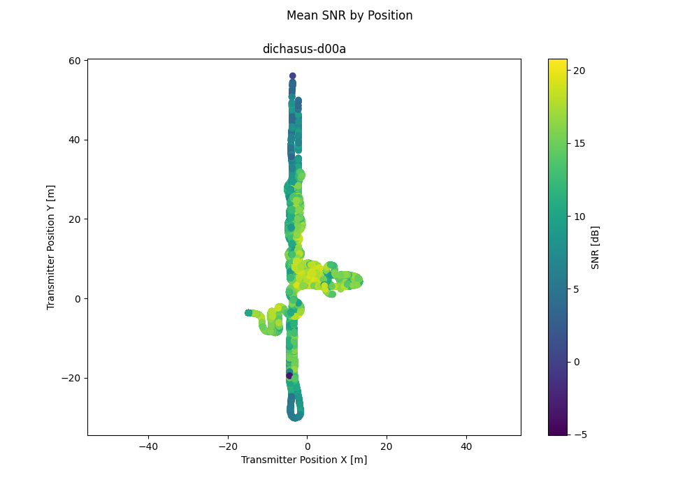
dichasus-d00a
dichasus-d00b
dichasus-d010
dichasus-d011

dichasus-d012

dichasus-d013
dichasus-d014
dichasus-d020
dichasus-d030
dichasus-d031
dichasus-d032

dichasus-d033
dichasus-d034
dichasus-d035
dichasus-d036

dichasus-d037
dichasus-d038
dichasus-d041
Derived Channel Statistics
Channel statistics such as delay spread, k-Factor and path loss exponent are a good way to characterize a wireless channel measurement and to parametrize a channel model. Using estimation algorithms contributed by Janina Sanzi, we automatically extract the following channel statistics from the measured datasets:
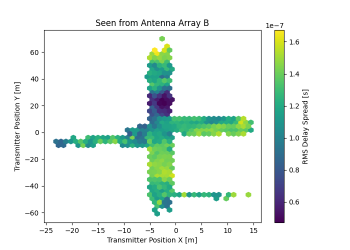
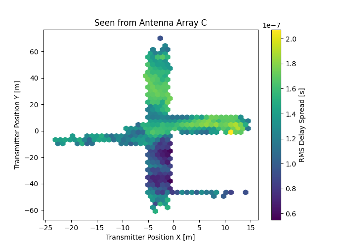
RMS Delay Spread
The delay spread of a wireless channel is inversely proportional to the channel's coherence bandwidth and indicates how "spread out" the lengths of the various multipath propagation paths are. For every datapoint, the delay spread can be characterized by its root mean square value and the resulting delay spreads can be plotted over the measurement area: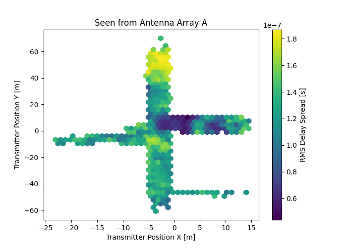
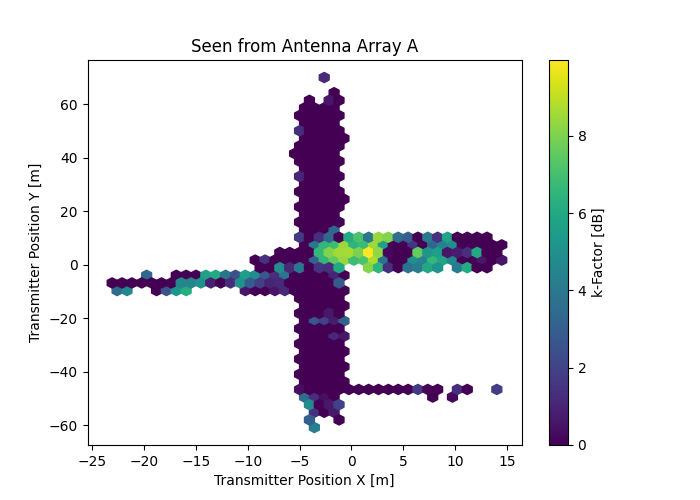
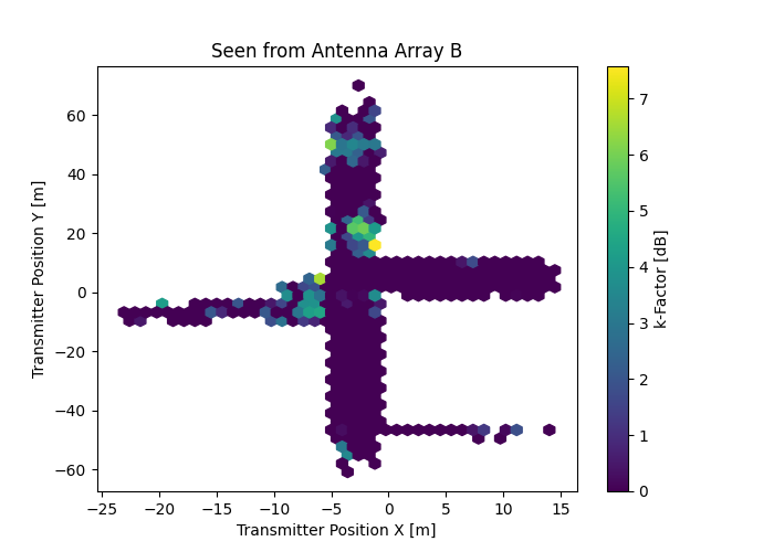
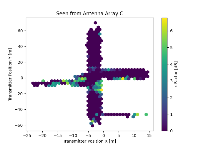
Rician K-Factor
The Rician K-factor is defined as the power ratio between dominant and diffuse component, usually expressed in decibels. We estimate the K-factor with a moment-method based on the distribution of of channel coefficient powers. The resulting K-Factors be plotted over the measurement area: