The Task
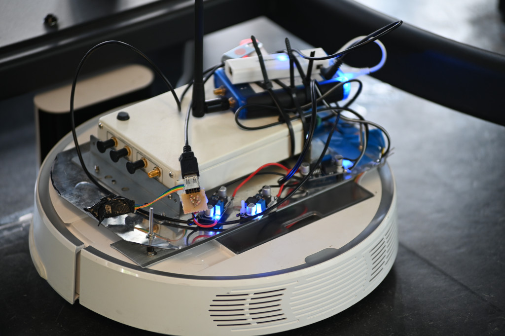
- A transmitter, continuously sending OFDM symbols, is mounted on top of a vacuum robot which performs multiple round trips inside the same area.
- The OFDM transmit signal is received by a massive MIMO 32-antenna array.
- The environment is assumed to be static for the duration of all robot round trips and we do not intend to generalize our model to different radio environments.
- Objective: Estimate the position of the transmitter inside the room (i.e., an indoor radio environment) purely based on the received OFDM signal.

The Dataset
For this tutorial, we use the dichasus-015x dataset.
DICHASUS uses a reference transmitter-based system architecture, which entails that measured phases may exhibit constant offsets caused by the reference transmitter channel.
Luckily, neural networks should be able to learn and adapt to such constant offsets, so, in contrast to classical methods, there is no need for us to compensate any of these offsets.
Before we can do any training, we must first load the dataset.
Conveniently, DICHASUS datasets are provided in the TFRecords file format, which makes loading them with TensorFlow particularly simple.
First, we download three robot round trips dichasus-0152.tfrecords, dichasus-0153.tfrecords and dichasus-0154.tfrecords:
!mkdir dichasus
!wget --content-disposition https://darus.uni-stuttgart.de/api/access/datafile/:persistentId?persistentId=doi:10.18419/darus-2202/2 -P dichasus # dichasus-0152
!wget --content-disposition https://darus.uni-stuttgart.de/api/access/datafile/:persistentId?persistentId=doi:10.18419/darus-2202/3 -P dichasus # dichasus-0153
!wget --content-disposition https://darus.uni-stuttgart.de/api/access/datafile/:persistentId?persistentId=doi:10.18419/darus-2202/4 -P dichasus # dichasus-0154
Next, we load the TFRecords files with TensorFlow. In the following, we use two complete robot round trips as training set and one round trip as test set:
import matplotlib.pyplot as plt
import matplotlib.cm as cm
import tensorflow as tf
import numpy as np
%matplotlib inline

training_files = ["dichasus/dichasus-0152.tfrecords", "dichasus/dichasus-0153.tfrecords"]
test_files = ["dichasus/dichasus-0154.tfrecords"]

def record_parse_function(proto):
	record = tf.io.parse_single_example(proto, {
		"csi": tf.io.FixedLenFeature([], tf.string, default_value = ''),
		"pos-tachy": tf.io.FixedLenFeature([], tf.string, default_value = '')
	})
	csi = tf.ensure_shape(tf.io.parse_tensor(record["csi"], out_type = tf.float32), (32, 1024, 2))
	pos_tachy = tf.ensure_shape(tf.io.parse_tensor(record["pos-tachy"], out_type = tf.float64), (3))

	# We only care about x/y position dimensions, z is always close to 0
	return csi, pos_tachy[:2]

training_set = tf.data.TFRecordDataset(training_files).map(record_parse_function)
test_set = tf.data.TFRecordDataset(test_files).map(record_parse_function)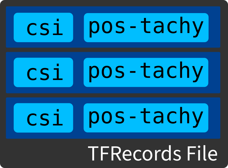
tf.train.Example key-value stores that we call datapoints.
In the code segment above, we only loaded the values of two keys, called features, into our variables training_set and test_set.
These two features are called csi and pos-tachy.
TFRecords files are a convenient way to load large datasets with TensorFlow without having to resort to writing custom import functions.
TensorFlow will be smart enough to automatically fetch data from storage whenever needed and, by default, does not cache the dataset in RAM.
Positioning "Ground Truth" Information
Let's start by visualizing the pos-tachy property.
It contains the three-dimensional position \((x, y, z)\) of the transmitter, as measured by a robotic total station (tachymeter), for any given datapoint.
Since tachymeters are very precise instruments, we can assume that this "ground truth" label is accurate down to a few millimeters.
The height coordinate \(z\) is close to \(0\) for the complete dataset, since the robot drives on (approximately) flat floor.
Visualizing \((x, y)\) coordinates on a plane should therefore give us a good impression of the robot positions.
In the following, we convert the coordinates stored in TensorFlow tensors to a large NumPy array "positions" which has dimensions \(N \times 3\), where \(N\) is the number of datapoints in the test_set.
positions = []
for datapoint in test_set:
	positions.append(datapoint[1].numpy())
positions = np.vstack(positions)

plt.figure(figsize=(5, 6))
plt.scatter(positions[:, 0], positions[:, 1])
plt.axis("equal")
plt.xlabel("x coordinate [m]")
plt.ylabel("y coordinate [m]")
plt.show()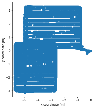
The resulting plot clearly shows that the robot mostly stayed inside two rectangular areas inside the room. According to the information on the dataset page, the receive antenna array was located at \((x, y, z) = (0, 0, 1)\) relative to the provided coordinates. We also have some datapoints where the robot is directly in front of / underneath this antenna array.
Channel Coefficients
The positions visualized in the previous section are fairly straightforward to understand.
The definition of instantaneous channel state iformation (CSI), on the other hand, is a bit more vague.
In our case, what we understand by "CSI" is the combination of OFDM subcarrier channel coefficients from all antennas with properties like signal-to-noise ratio (SNR) and carrier frequency offset (CFO).
In this tutorial, we will focus purely the channel coefficients.
For a fixed time instance (i.e., for one datapoint), the dichasus-015x dataset contains \(M = 32\) channel coefficient vectors \(\mathbf h_m \in \mathbb C^{N_\mathrm{sub}}\), one for each antenna \(m = 0, \ldots, M-1\).
Each channel coefficient vector, in turn, contains \( N_\mathrm{sub} = 1024 \) channel coefficients, one per subcarrier.
Channel coefficients are complex numbers, where the amplitude corresponds to the attenuation experienced by the particular subcarrier and the argument corresponds to the phase shift.
In DICHASUS datasets, these are stored in real part / imaginary part format.
Thus, the channel coefficient tensor for each datapoint has dimensions \(M \times N_\mathrm{sub} \times 2\).
The following code snippet will choose a random datapoint and plot amplitude and phase of all corresponding channel coefficient vectors \(\mathbf h_m \in \mathbb C^{N_\mathrm{sub}}, ~ m = 0, \ldots, M-1\) over the subcarrier index \( i = 0, \ldots, N_\mathrm{sub} - 1 \). For some datapoints, the measured channel coefficient vectors contain clearly visible spectral notches, which are due to frequency-selective fading:
csi_tensor = next(iter(test_set.shuffle(1000).take(1)))[0]

plt.figure(figsize = (10, 7))
plt.subplot(211)
plt.title("Channel State Information: Channel Coefficients")
plt.xlabel("Subcarrier $i$")
plt.ylabel("Referenced channel coeff.,\n abs. value $|h_i|_{dB}$ [dB]")
for antenna_csi in tf.unstack(csi_tensor):
	plt.plot(10 * np.log10(np.abs(np.fft.fftshift(antenna_csi[:,0]**2 + antenna_csi[:,1]**2))))

plt.subplot(212)
plt.xlabel("Subcarrier $i$")
plt.ylabel("Referenced channel coeff.,\nphase shift $arg(h_i)$")
for antenna_csi in tf.unstack(csi_tensor):
	plt.plot(np.unwrap(np.fft.fftshift(np.arctan2(antenna_csi[:,1], antenna_csi[:,0]))))

plt.show()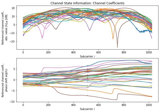
Feature Engineering and Input Normalization
Our goal is to generate positions estimates \( (\hat x, \hat y) \) from CSI using a neural network. In theory, we could provide all \( M \times N_\mathrm{sub} \) "raw" channel coefficients to our neural network and let it directly estimate \( (\hat x, \hat y) \) from this raw data. This approach, while it would certainly produce useful results, has the drawback of high neural network complexity: For every datapoint, we have \( M \cdot N_\mathrm{sub} \cdot 2 = 32 \cdot 1024 \cdot 2 = 65536 \) input values to the neural network. Such an excessive amount of input parameters unnecessarily increases neural network complexity and therefore training time. Since channel coefficients of neighboring subcarriers are highly correlated, an obvious simplification is to average neighboring subcarriers. In the following, we simply compute averages over chunks of \( 32 \) subcarriers, reducing the number of input parameters to \( 32 \cdot 32 \cdot 2 = 2048 \).def get_feature_mapping(chunksize = 32):
def compute_features(csi, pos_tachy):
assert(csi.shape[1] % chunksize == 0)
featurecount = csi.shape[1] // chunksize
csi_averaged = tf.stack([tf.math.reduce_mean(csi[:, (chunksize * s):(chunksize * (s + 1)), :], axis = 1) for s in range(featurecount)], axis = 1)
return csi_averaged, pos_tachy
return compute_features
training_set_features = training_set.map(get_feature_mapping(32))
test_set_features = test_set.map(get_feature_mapping(32))
training_set_features = training_set_features.shuffle(buffer_size = 100000)
test_set_features = test_set_features.shuffle(buffer_size = 100000)Neural Network Architecture
The design of neural networks is almost a whole engineering discipline on its own. With convolutional networks, residual networks, transformers and many other models to chose from, things can quickly get confusing. Within the scope of this tutorial, however, we don't care so much about finding the optimal neural network for positioning, just as long as we can demonstrate that a neural-network based approach works at all. Therefore, we resort to the simplest of all neural network architectures: A dense network.
Even with the choice of neural network type pinned down, we still have several degrees of freedom:
- Activation function: We chose ReLU, which is arguably the most popular activation function. Among other benefits, it is easy and fast to compute.
- Number of layers: We should provide enough hidden layers so that our model can capture the nonlinearity of the input-output relationship sufficiently well, but not unnecessarily increase network complexity with more layers. In this tutorial, we assume that three hidden layers should be sufficient.
- Size of hidden layers: Again, there only exist some rough "rules of thumb" for this choice; the number of neurons in hidden layers should be somewhere in between the size of the input layer and the size of the ouput layer. In the following, we chose the size of hidden layers so that the width of the layers decreases from input to output.
Another issue is feeding complex-valued channel coefficients into a neural network that only deals with real numbers. One approach might be to separate the channel coefficients into magnitude and phase. This encoding, however, is not a good choice for neural networks: If represented in radians, the phase values \( \varphi \) and \( \varphi + 2 \pi \) denote the exact same angle; the neural network, however, would output different results for these inputs. Even worse, the sudden wrap-around in phase from \( 2 \pi \, \mathrm{rad} \) to \( 0 \, \mathrm{rad} \) suggests a discontinuity in the input space when really, there is none, which negatively impacts training performance. Providing complex numbers in real / imaginary part format, just like they are stored in the TFRecords file, is a much better-suited representation that we will use in the following.

nn_input = tf.keras.Input(shape=(32,32,2), name="input")

nn_output = tf.keras.layers.Flatten()(nn_input)
nn_output = tf.keras.layers.Dense(units=512, activation="relu")(nn_output)
nn_output = tf.keras.layers.Dense(units=128, activation="relu")(nn_output)
nn_output = tf.keras.layers.Dense(units=128, activation="relu")(nn_output)
nn_output = tf.keras.layers.Dense(units=2, activation="linear", name="output")(nn_output)

nn = tf.keras.Model(inputs=nn_input, outputs=nn_output, name="localization")
Training
Before we can train this neural network to perform localization, we first need to decide on which loss function to use. Since 2D positioning is a regression problem, a mean squared error (MSE) loss is a reasonable choice for a loss function. Again, for the other hyperparameters such as learning rate schedule, number of epochs and batch size, we just choose some reasonable values without further consideration or optimization:nn.compile(optimizer=tf.keras.optimizers.Adam(), loss=tf.keras.losses.MeanSquaredError())
batch_sizes = [32,64,256,1024,4096]
for b in batch_sizes:
dataset_batched = training_set_features.batch(b)
test_set_batched = test_set_features.batch(b)
print("\nTraining with batch size:", b)
nn.fit(dataset_batched, epochs=20, validation_data=test_set_batched)Evaluation
At this point, we have a model that should be able to estimate the transmitter's position purely based on CSI data. To evaluate this neural network, we will use the third round trip of the vacuum robot downloaded earlier, i.e., a test set with datapoints that the network has never seen before. Before we can visualize the localization accuracy with some plots, we must first collect the position predictions of the model for all datapoints in the test set:true_positions = []
predictions = []
for channel_coeffs, positions in test_set_batched:
true_positions.append(positions)
predictions.append(nn.predict(channel_coeffs))
true_positions = np.vstack(true_positions)
predictions = np.vstack(predictions)
error_vectors = predictions - true_positions
absolute_errors = np.sqrt(error_vectors[:,0]**2 + error_vectors[:,1]**2)plt.figure(figsize=(12,3))
plt.title('Error distance distibution')
plt.xlabel('error distance in m')
plt.ylabel('occurences')
plt.hist(absolute_errors, bins=100, range=(0, 1))
plt.show()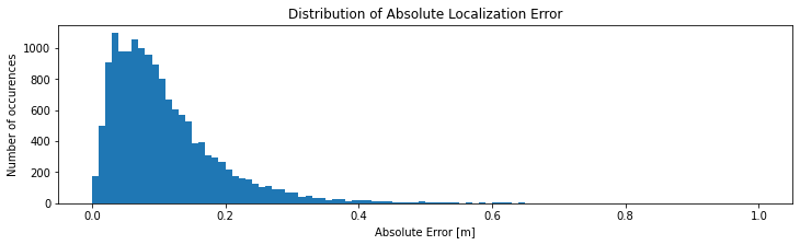
plt.figure(figsize=(12, 12))

plt.hexbin(true_positions[:,0], true_positions[:,1], C = absolute_errors, gridsize = 35, cmap = cm.jet, vmin = 0, vmax = 0.5)
plt.axis("equal")
cb = plt.colorbar()
cb.set_label("Absolute Error [m]", fontsize = 14)
plt.xlabel("x [m]", fontsize = 14)
plt.ylabel("y [m]", fontsize = 14)
plt.show()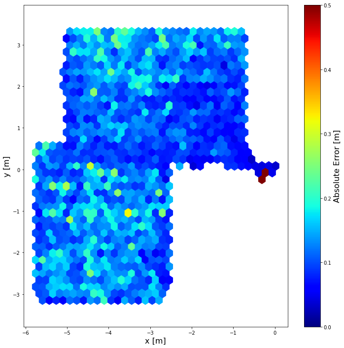
Generalizability
Clearly, for a well-defined scenario with CSI datapoints available for many locations inside the room, the neural network can learn the relationship between channel coefficients and transmitter position. However, if we had labeled traning data only for a small section of the room, e.g., only at the area's perimeter, would this approach still work? In other words, does the neural network just do "fingerprinting" (associate test set datapoints with similar datapoints it has seen before during training, similar to k-Nearest Neighbor Regression), or has it actually learned some properties of the antennas and the physical environment?
A detailed investigation of this question is outside the scope of this tutorial, but experiments have shown that this approach indeed does not generalize to previously unseen areas in the measurement environment. Different position estimation techniques based on the same dataset, such as angle estimation, yield results which generalize much better than the naive approach presented here.
Conclusion
With DICHASUS datasets, we demonstrated that deep neural network-based indoor positioning based on CSI data is feasible. Some important lessons for using DICHASUS datasets were learned along the way:- DICHASUS datasets are provided in the TFRecords format, which is particularly suitable for deep-learn with TensorFlow, but which can also be used in many other applications.
- In the context of DICHASUS, CSI refers primarily to channel coefficients for all antennas and all OFDM subcarriers
- DICHASUS datasets also contain precise "ground truth" positioning information
- In many deep learning applications with DICHASUS datasets, it is not necessary to find the optimal neural network architecture - it is much more important to formulate the right optimization problem.
- While the naive approach to CSI-based indoor positioning with dense neural networks produces accurate results, it does not generalize well to previously unseen transmitter positions.