dichasus-dxxx-complete Dataset: Outdoor - Three arrays distributed along the facade
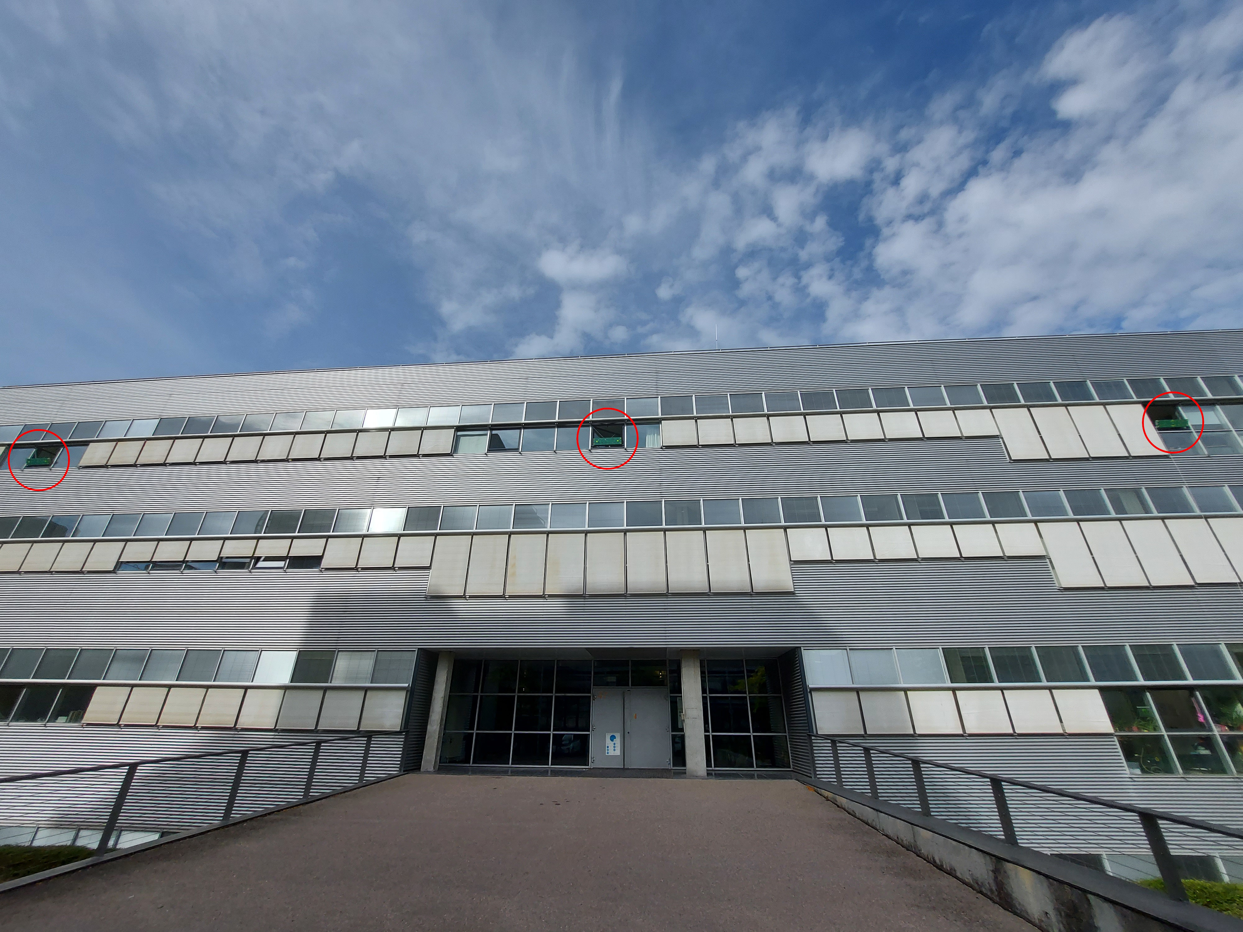
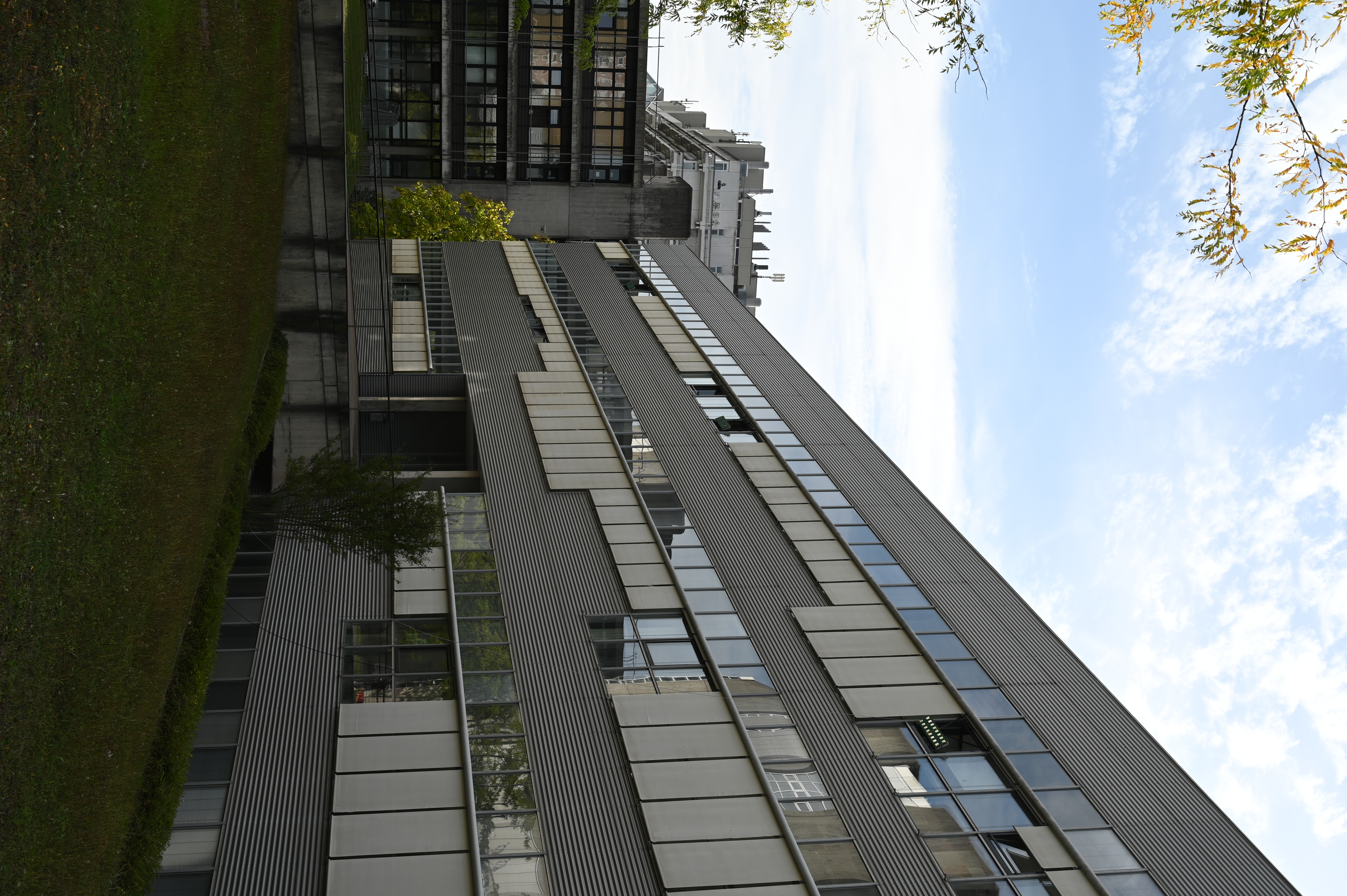
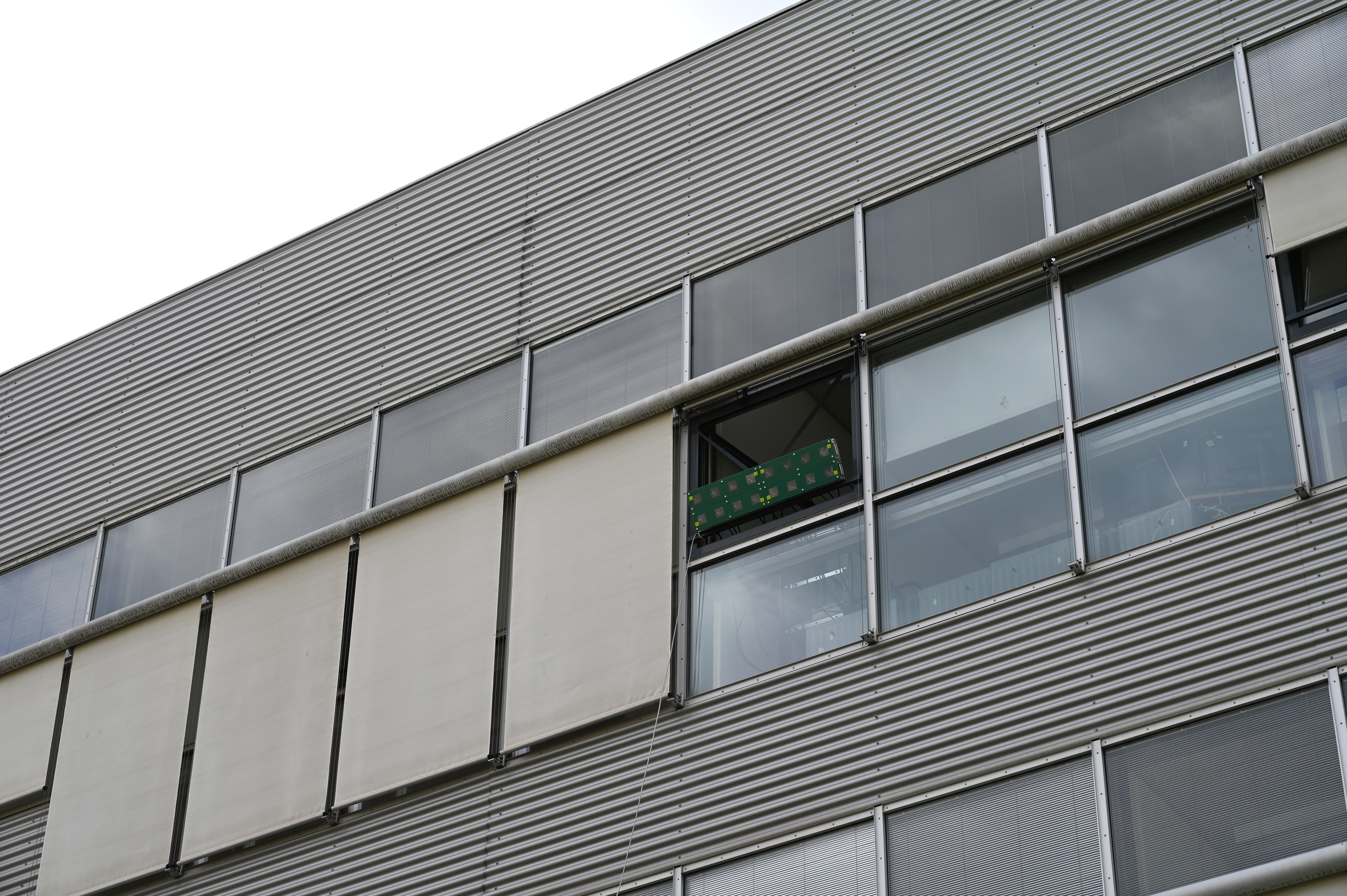
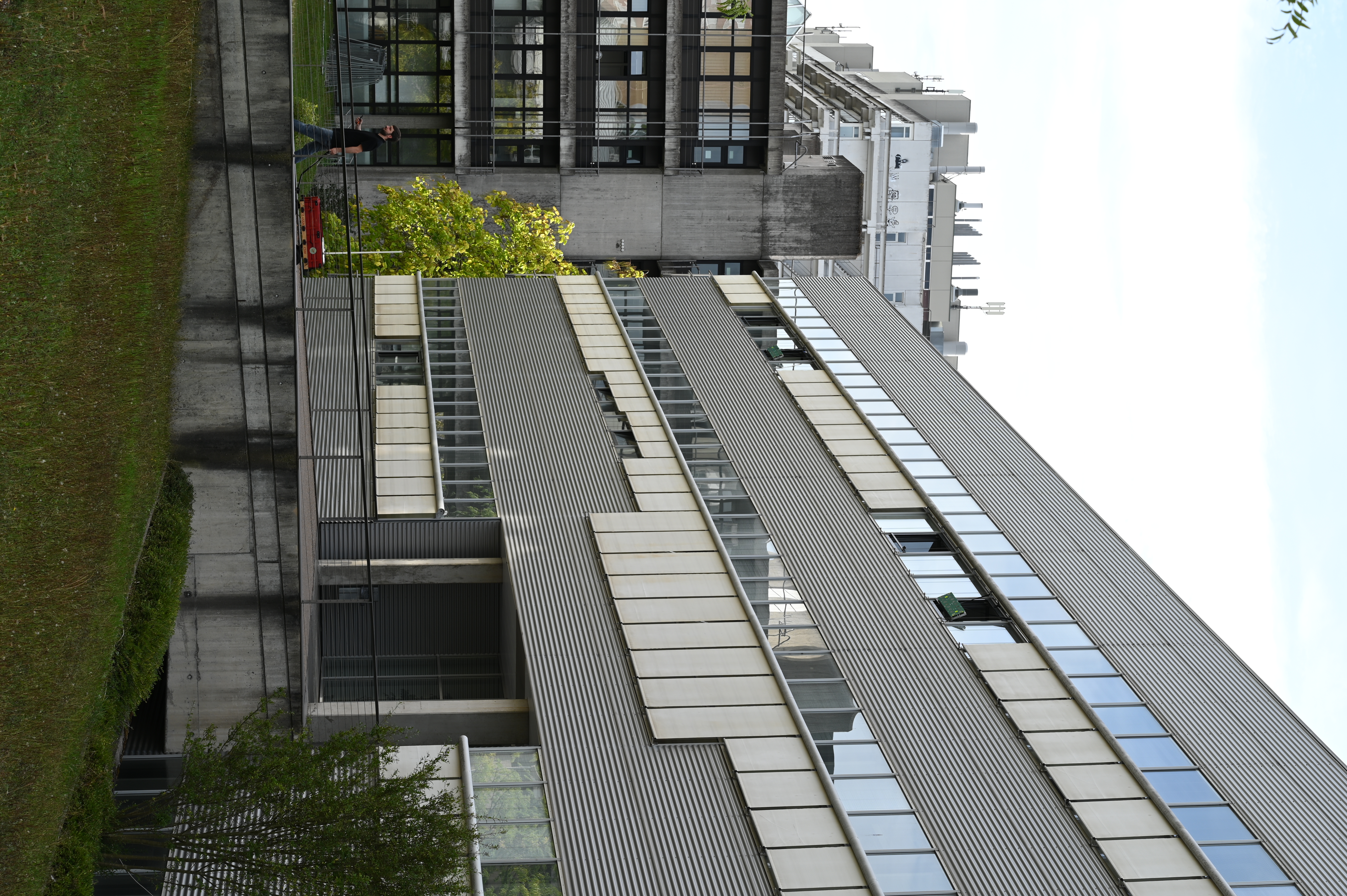
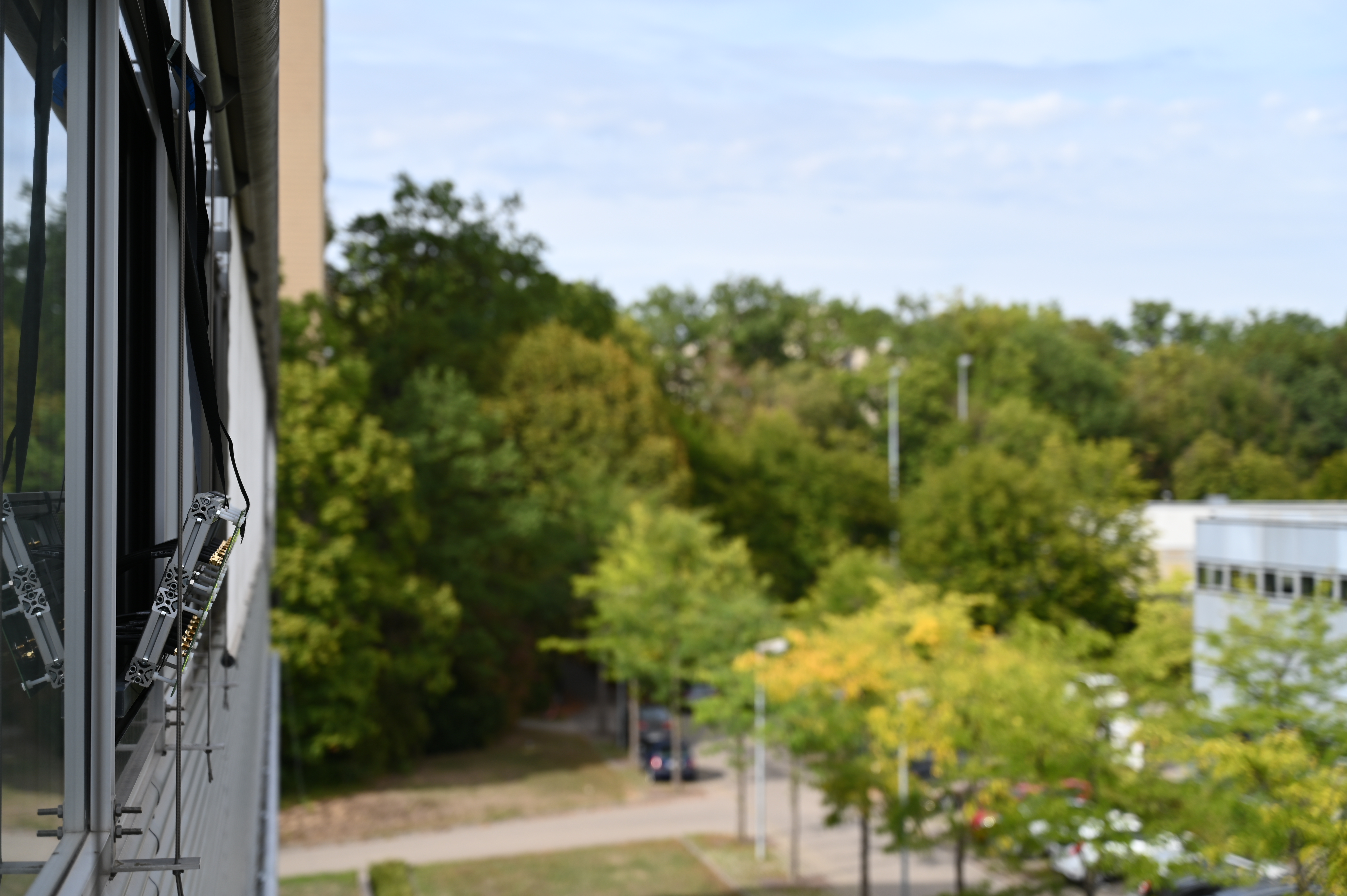
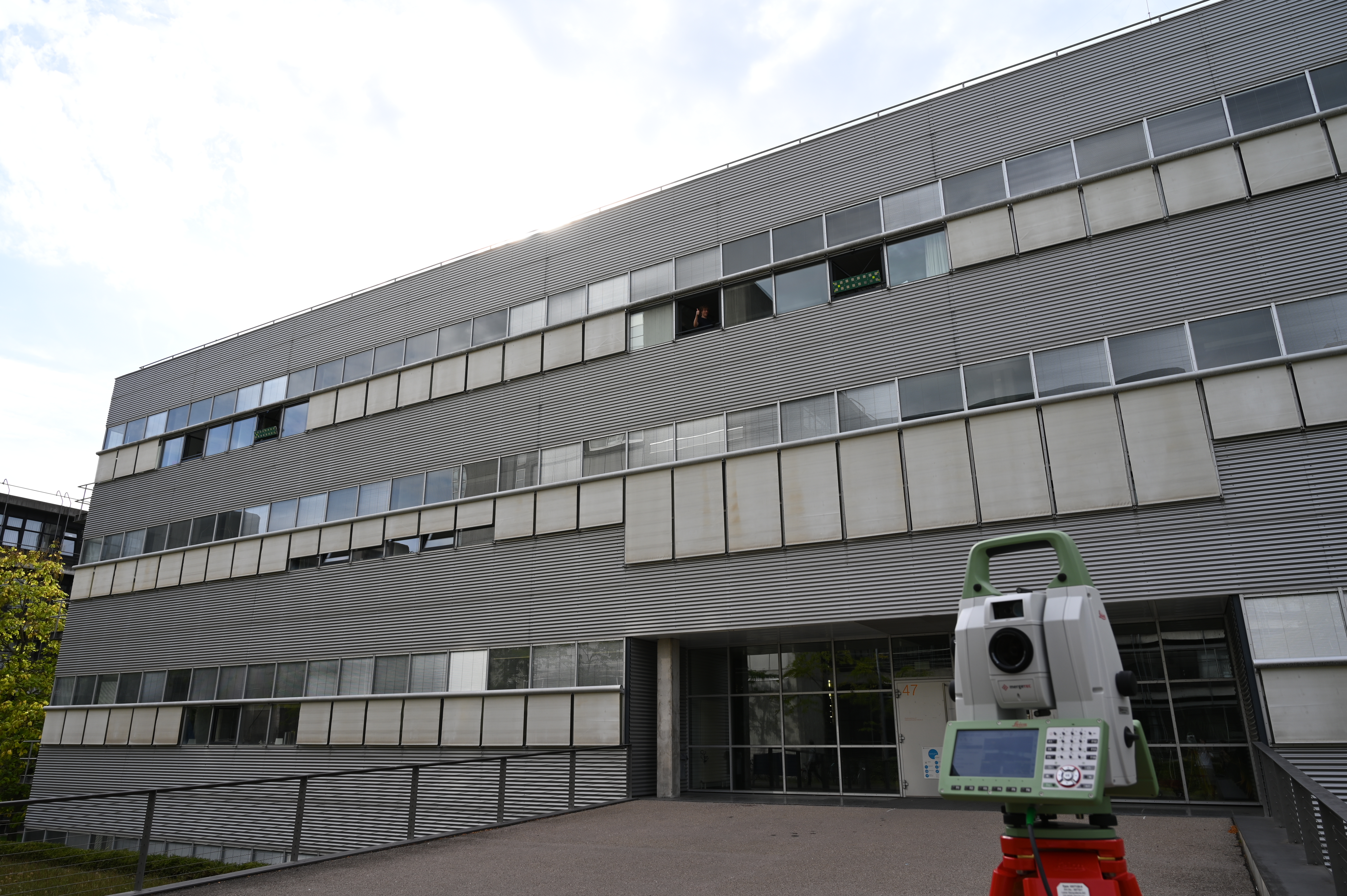
Three 2 x 8 antenna arrays are distributed along the facade of a building, separated by up to 35m.
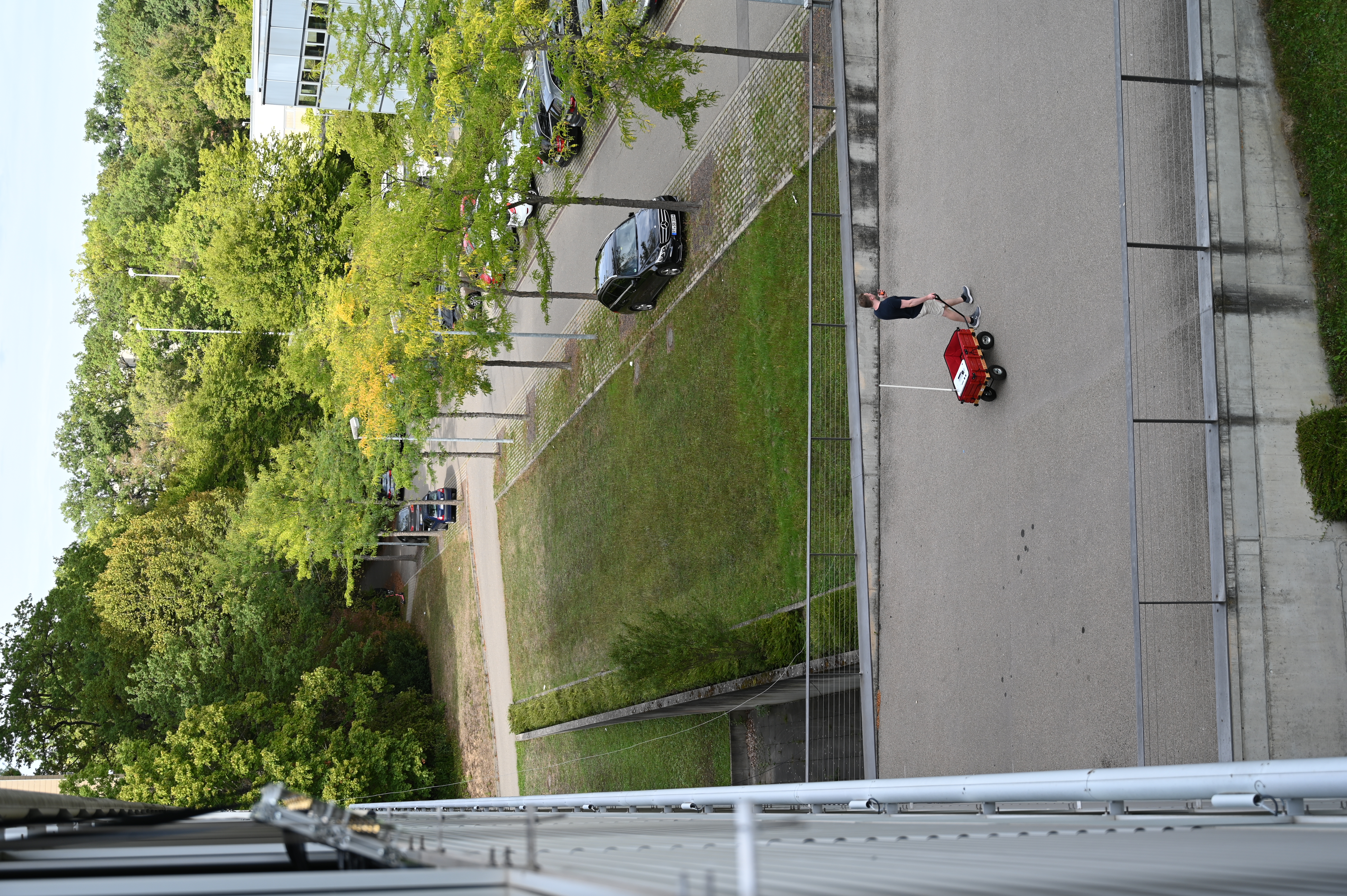
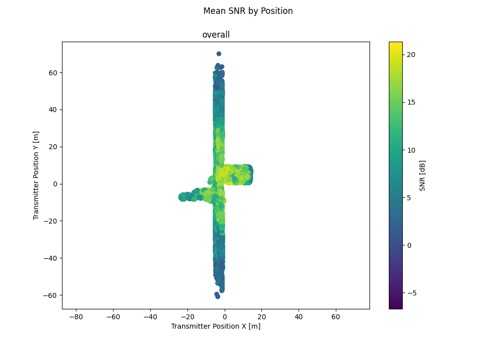
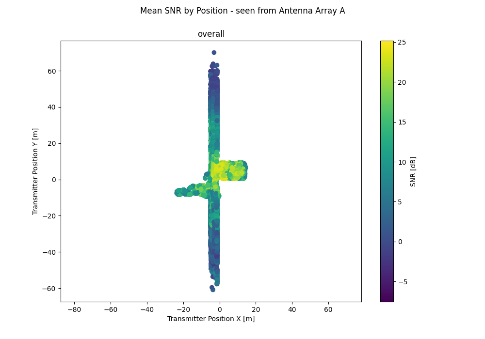
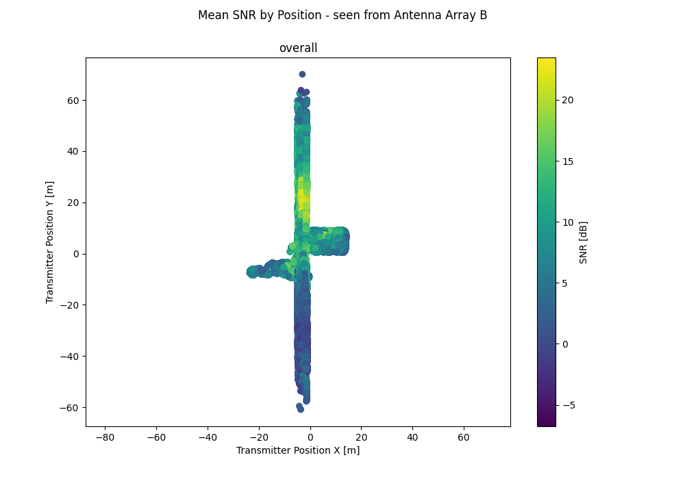
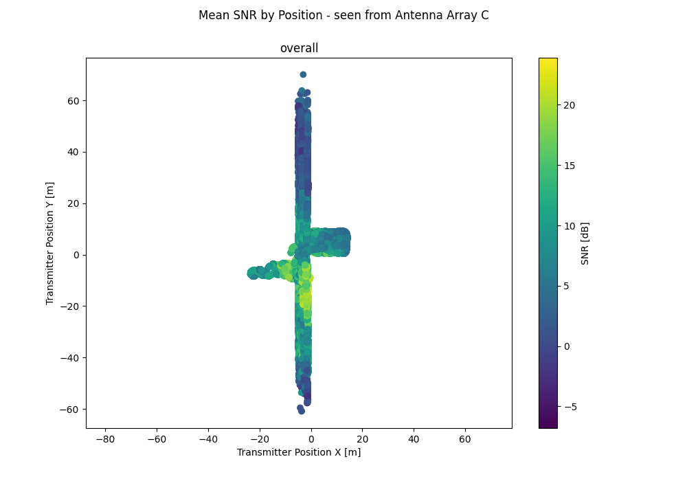
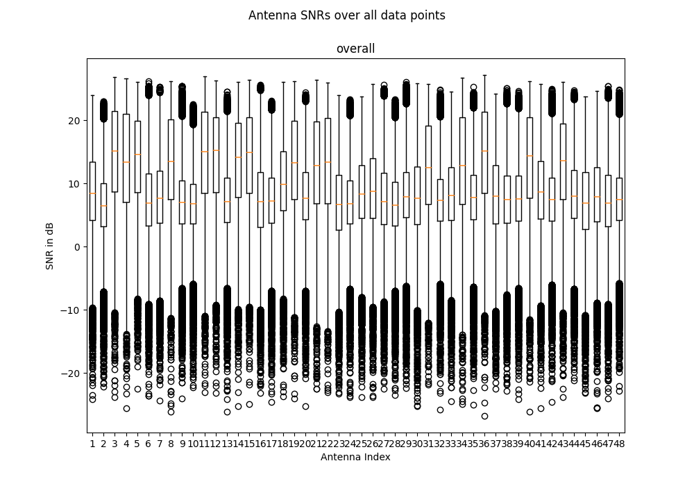
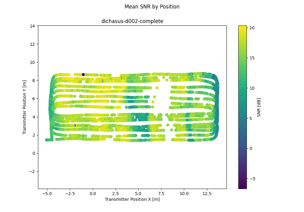
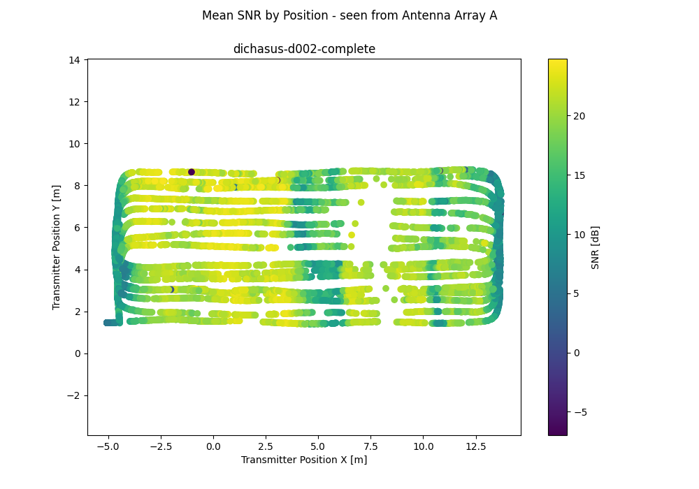
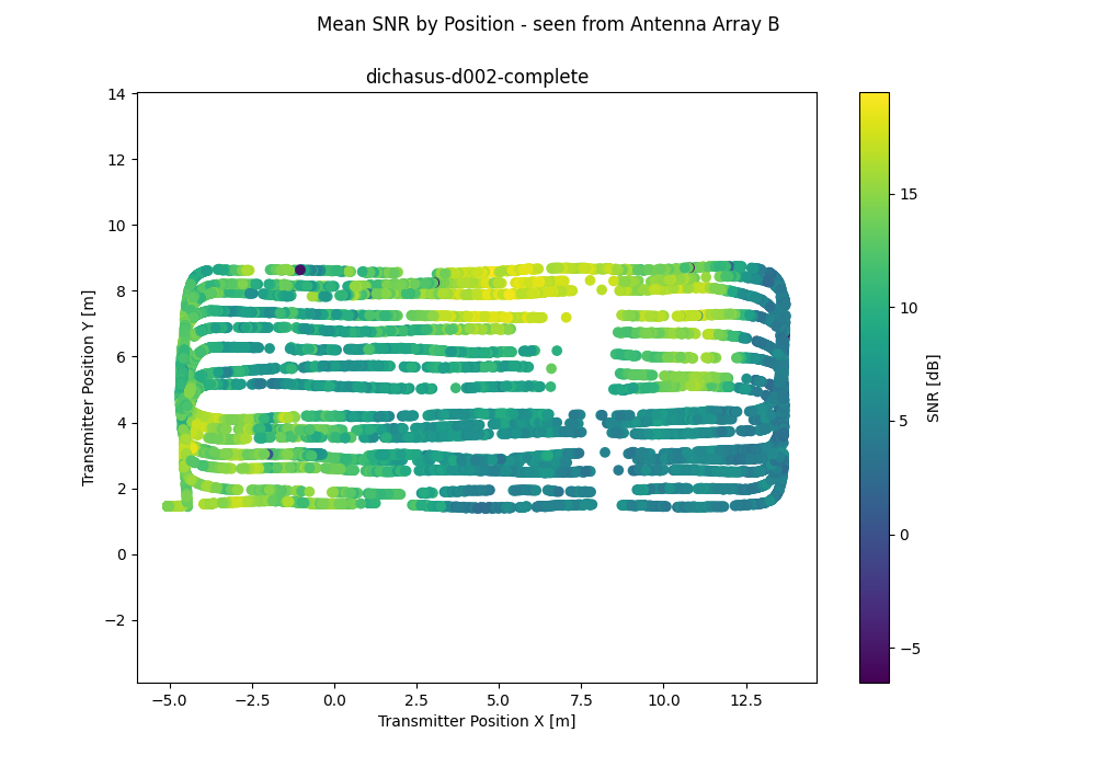
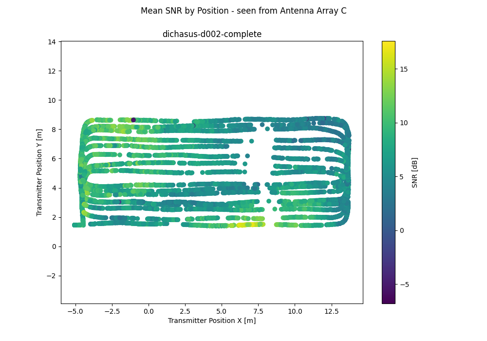
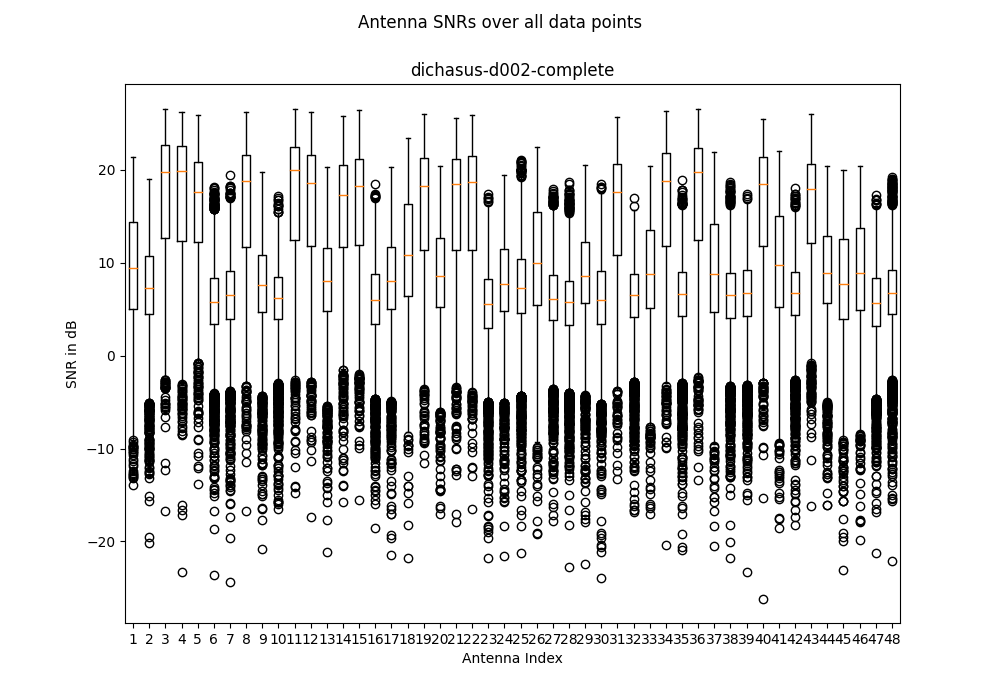
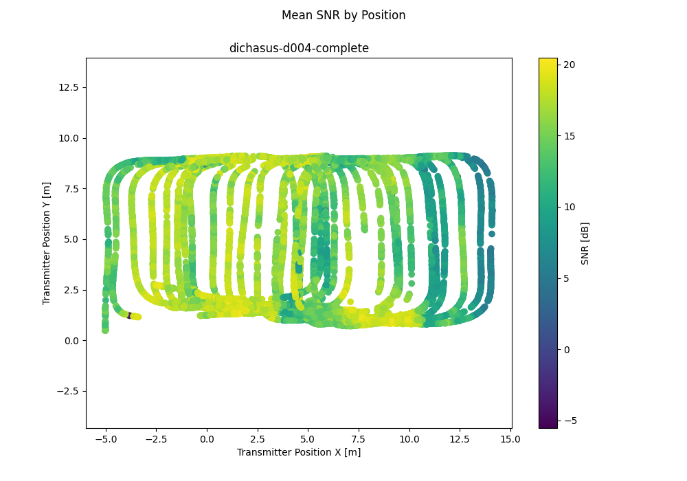
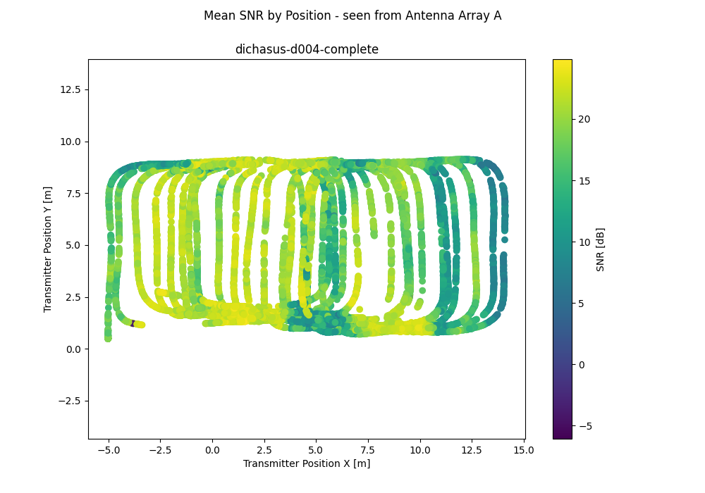
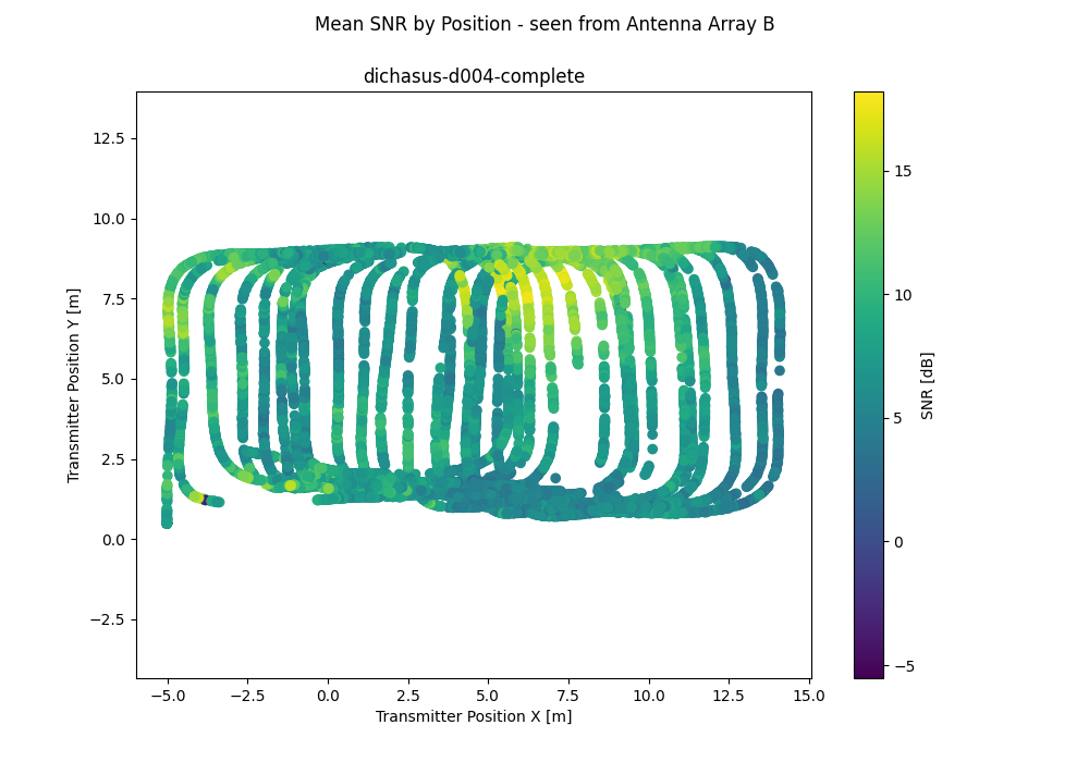
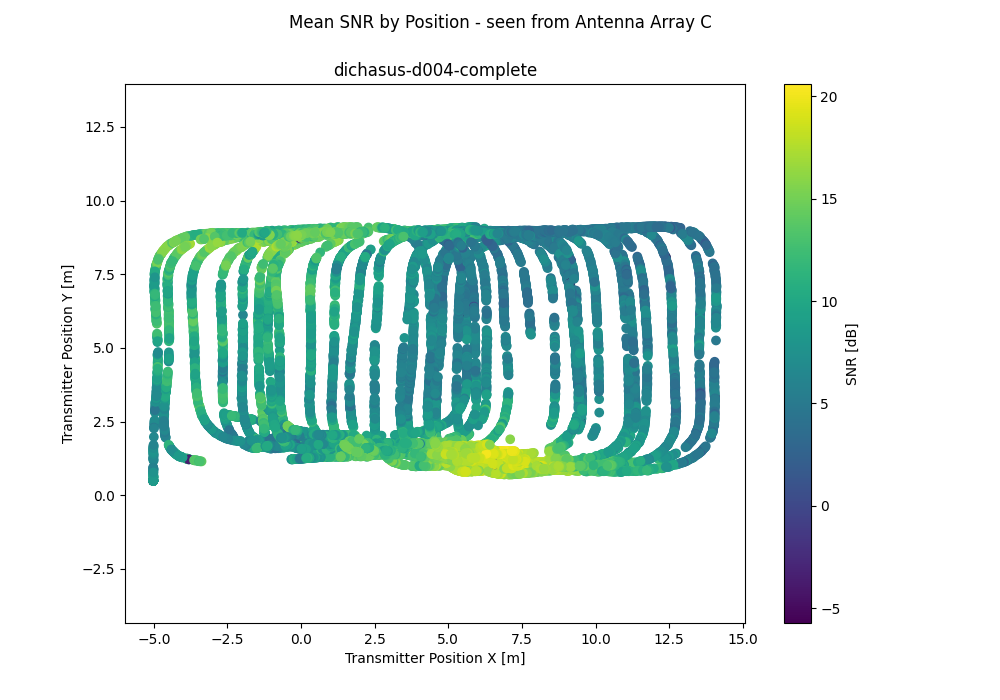
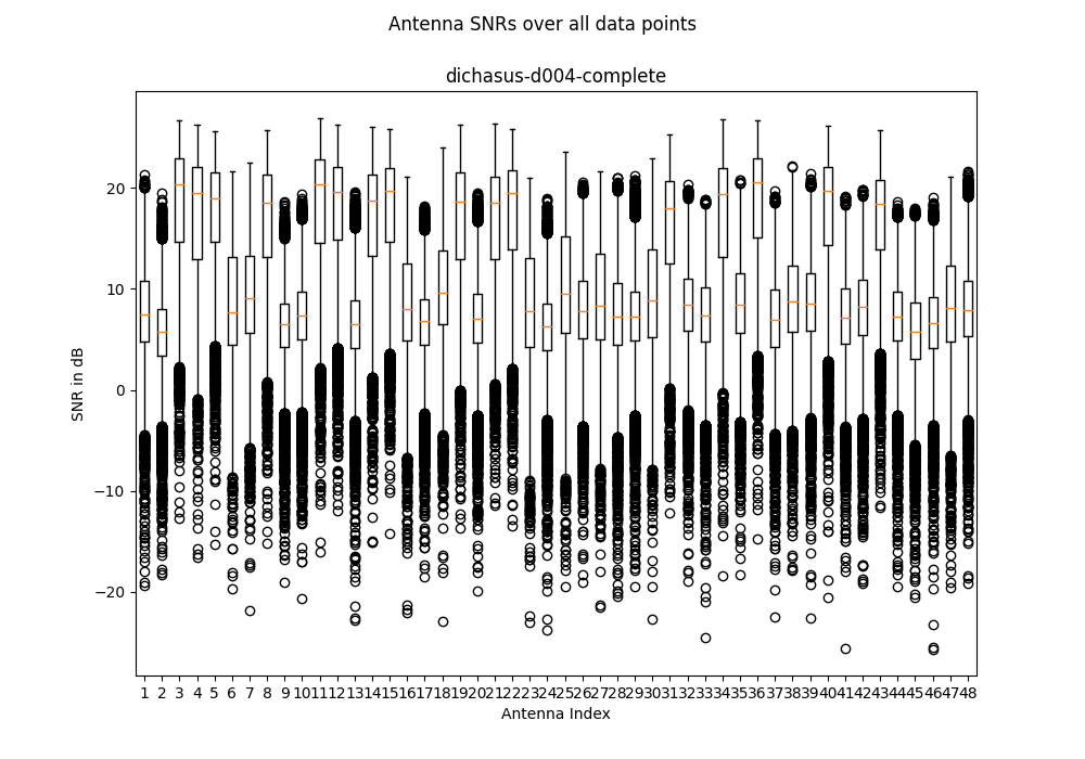
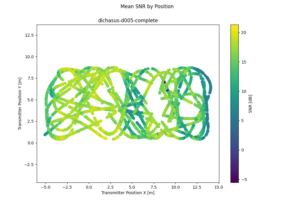
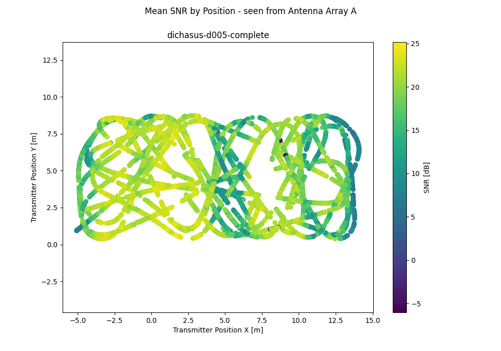
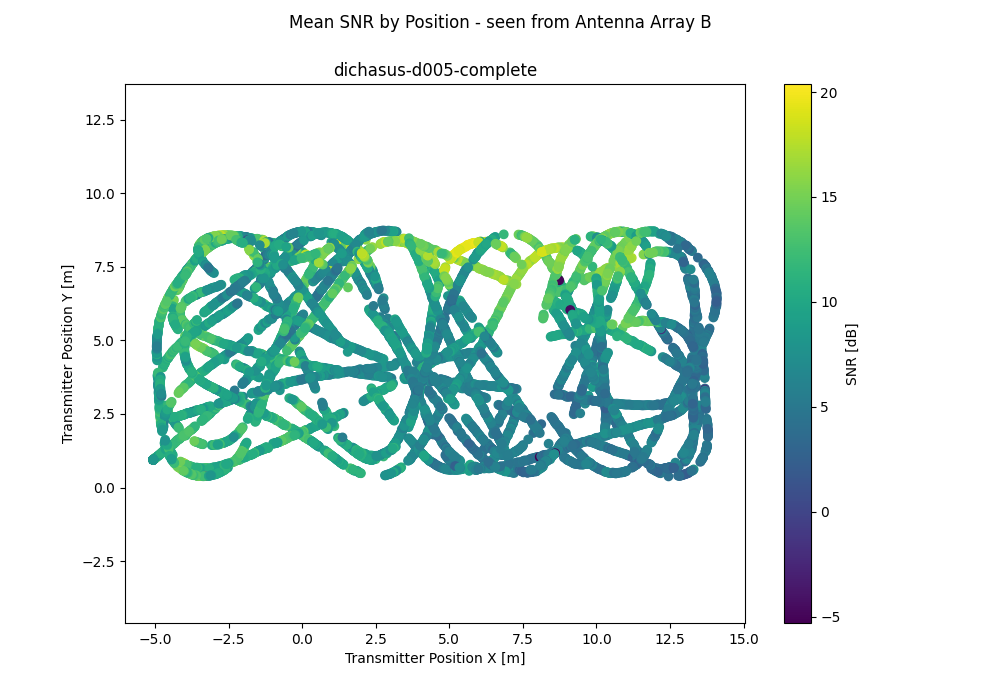
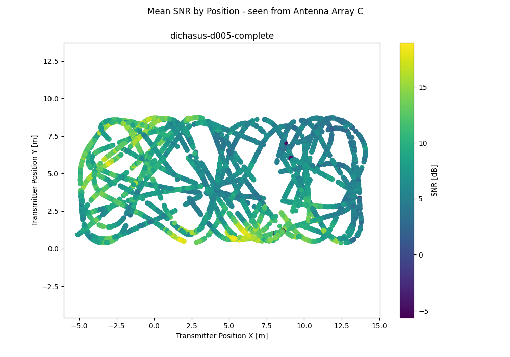
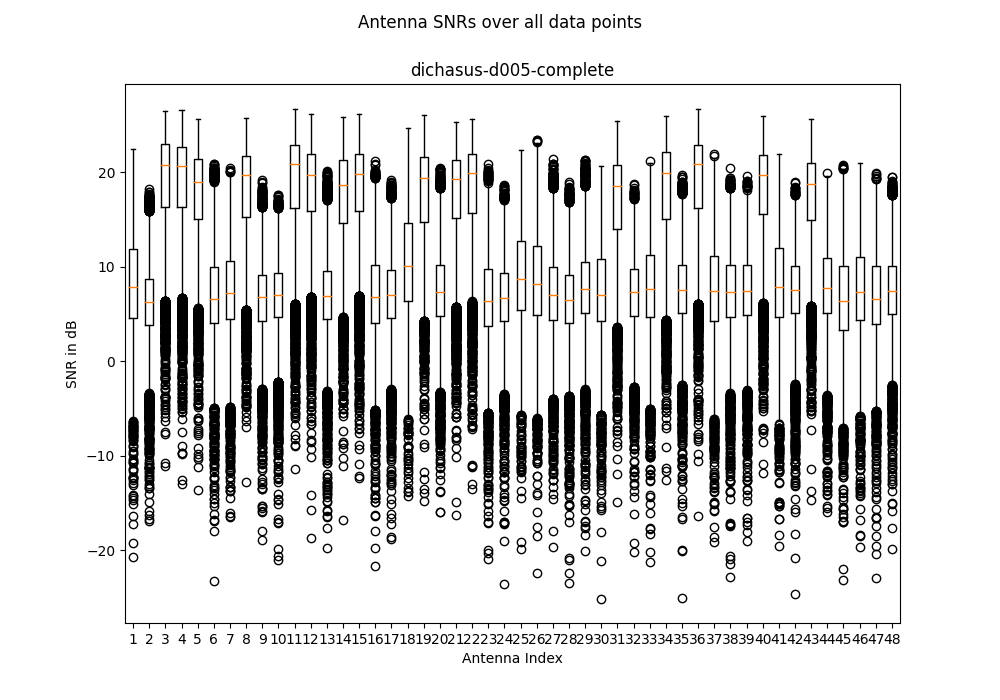
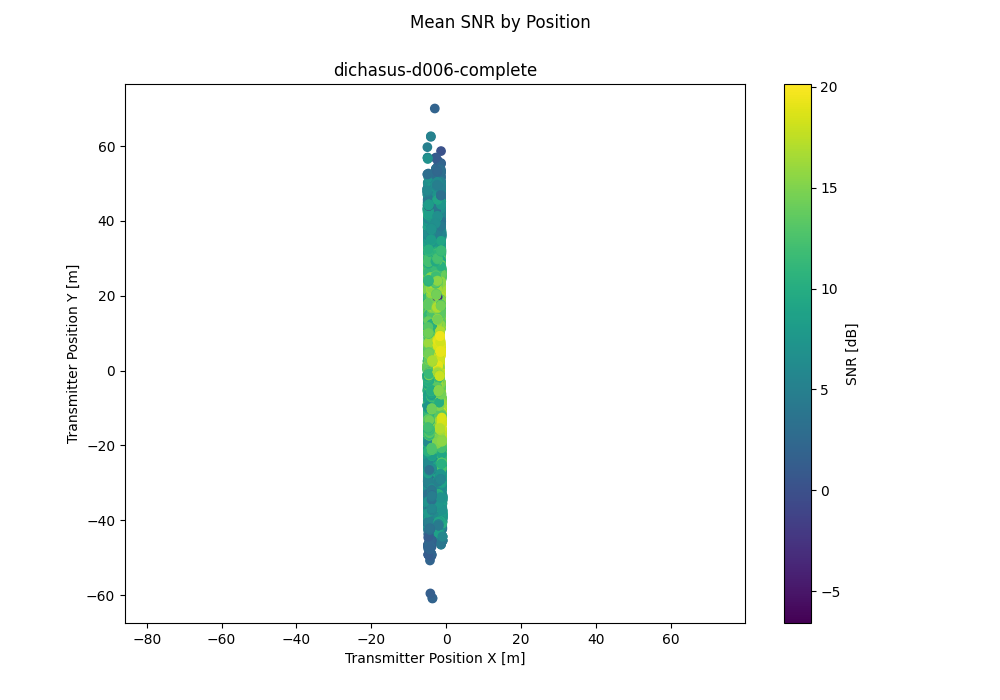
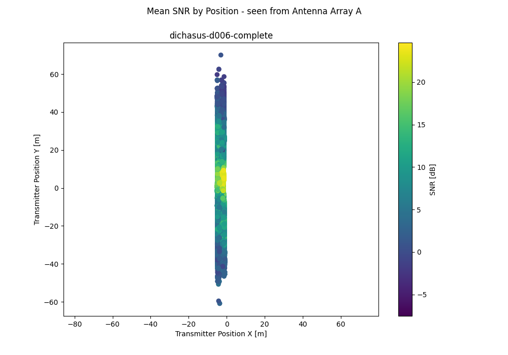
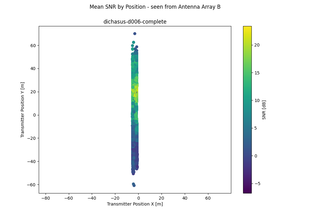
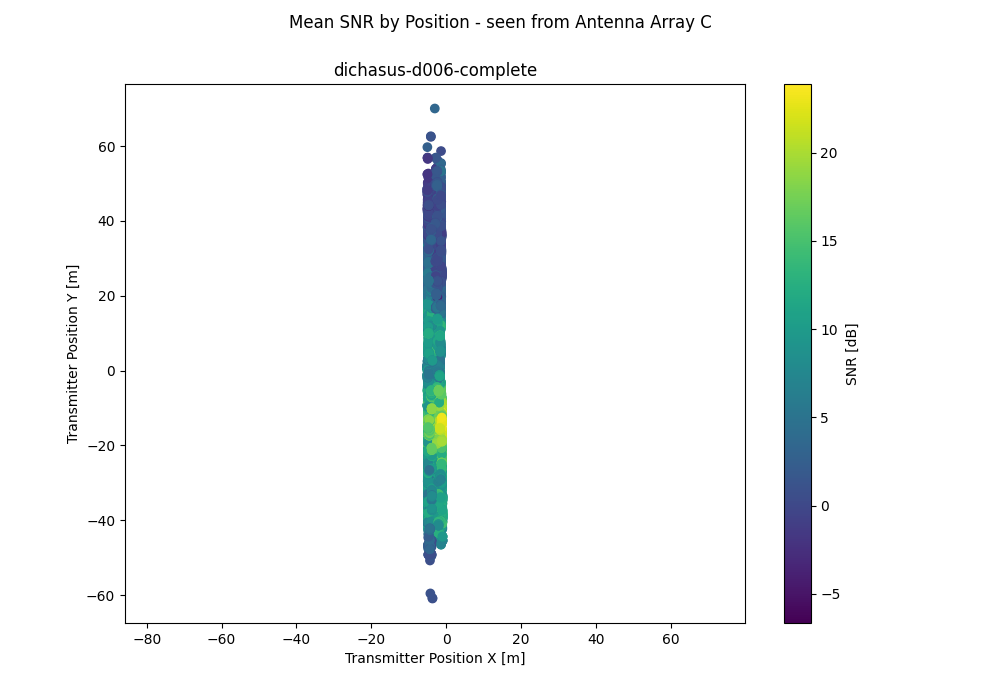
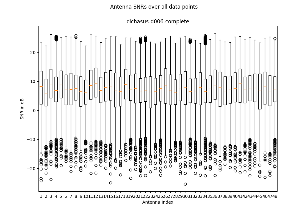
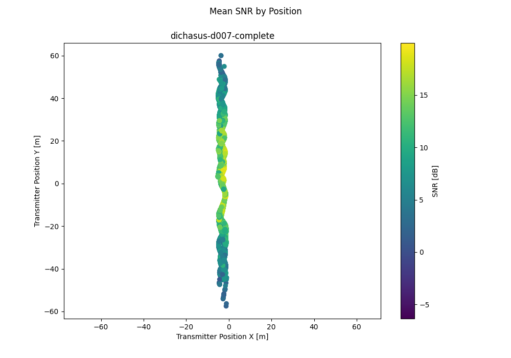
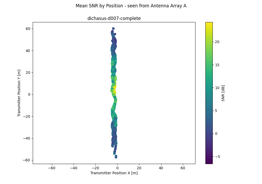
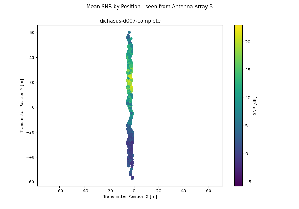
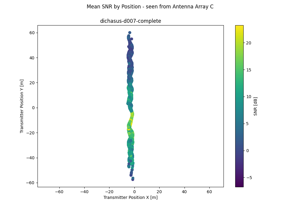
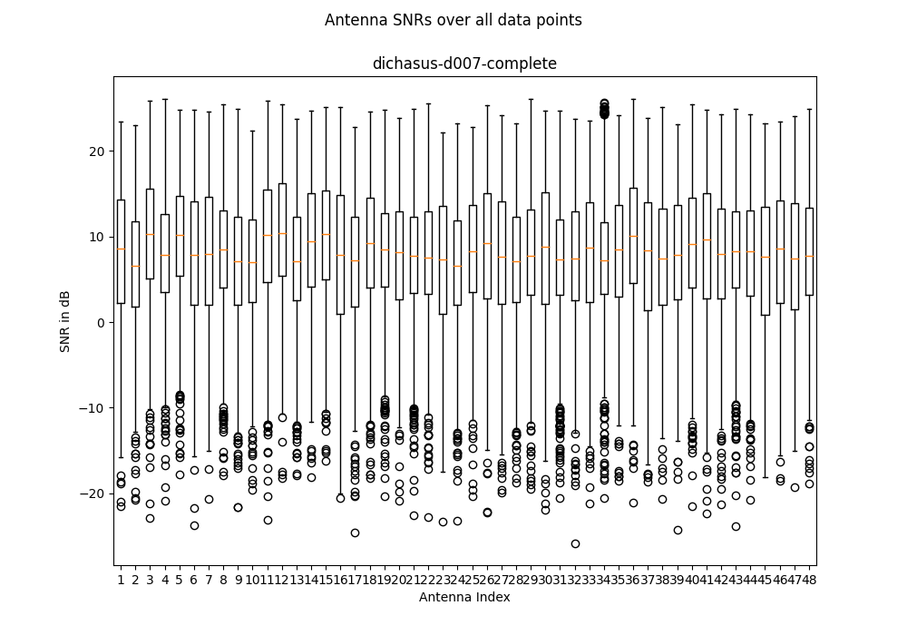
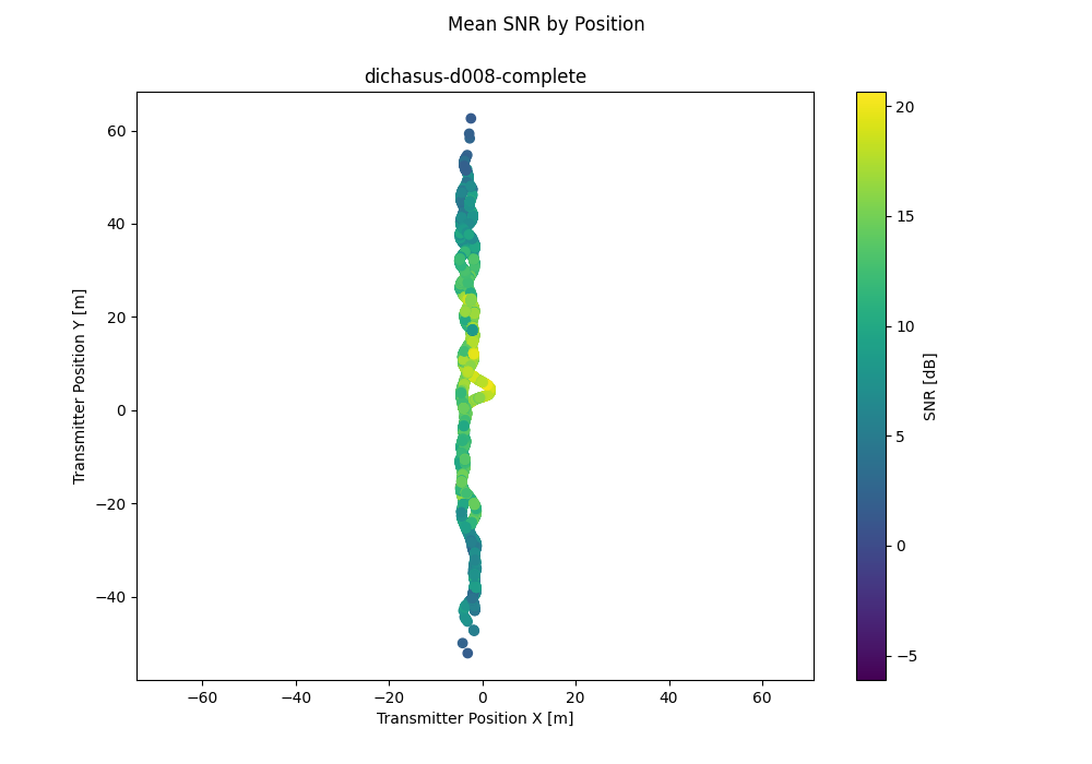
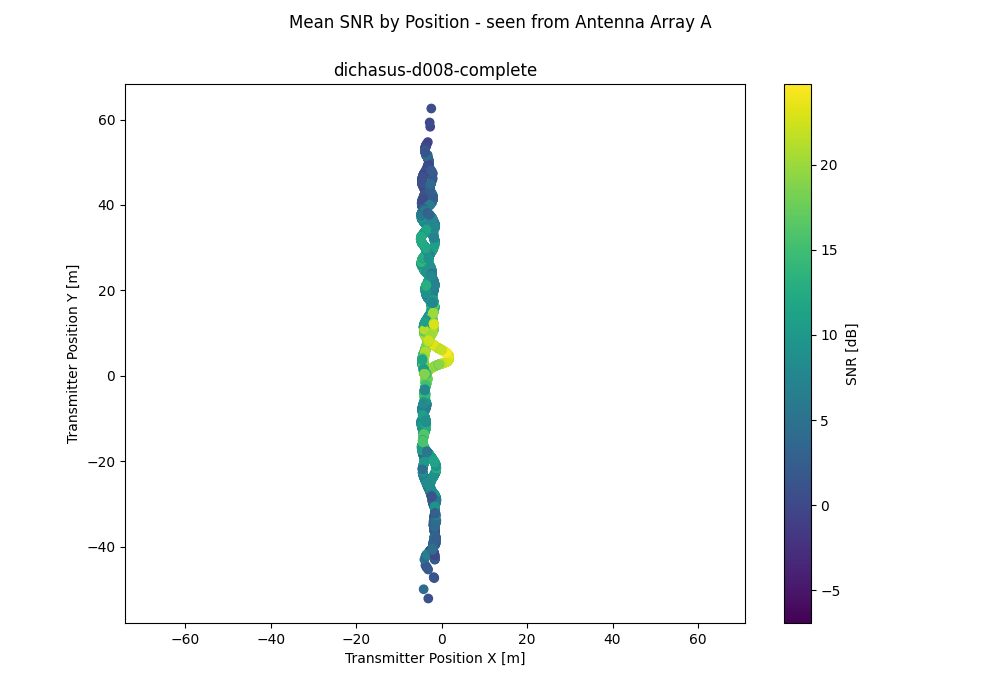
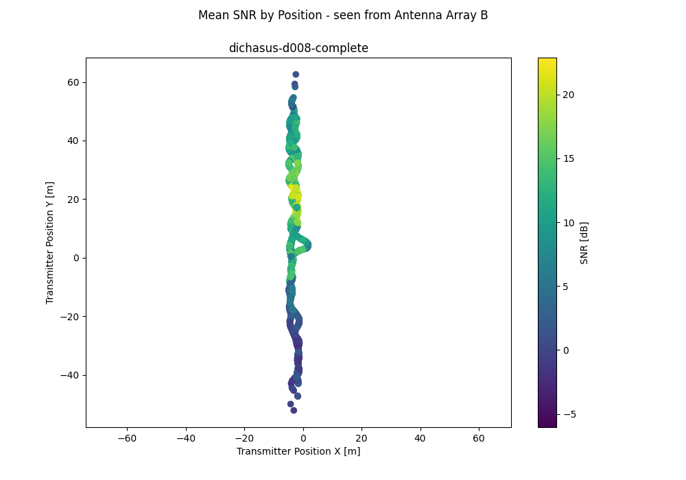
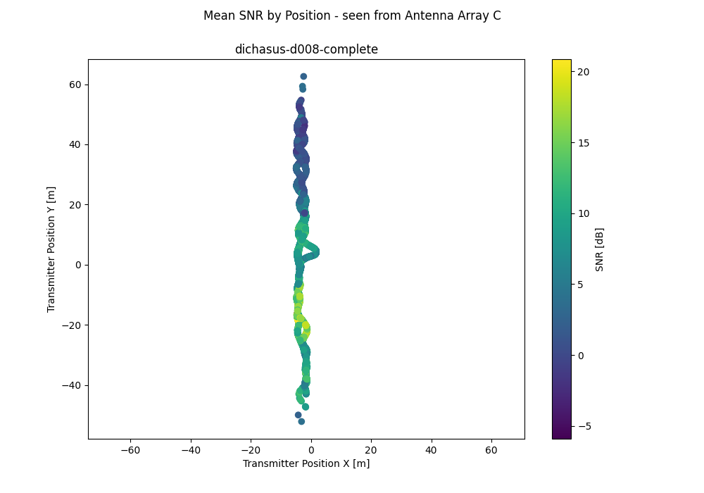
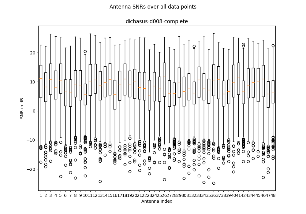
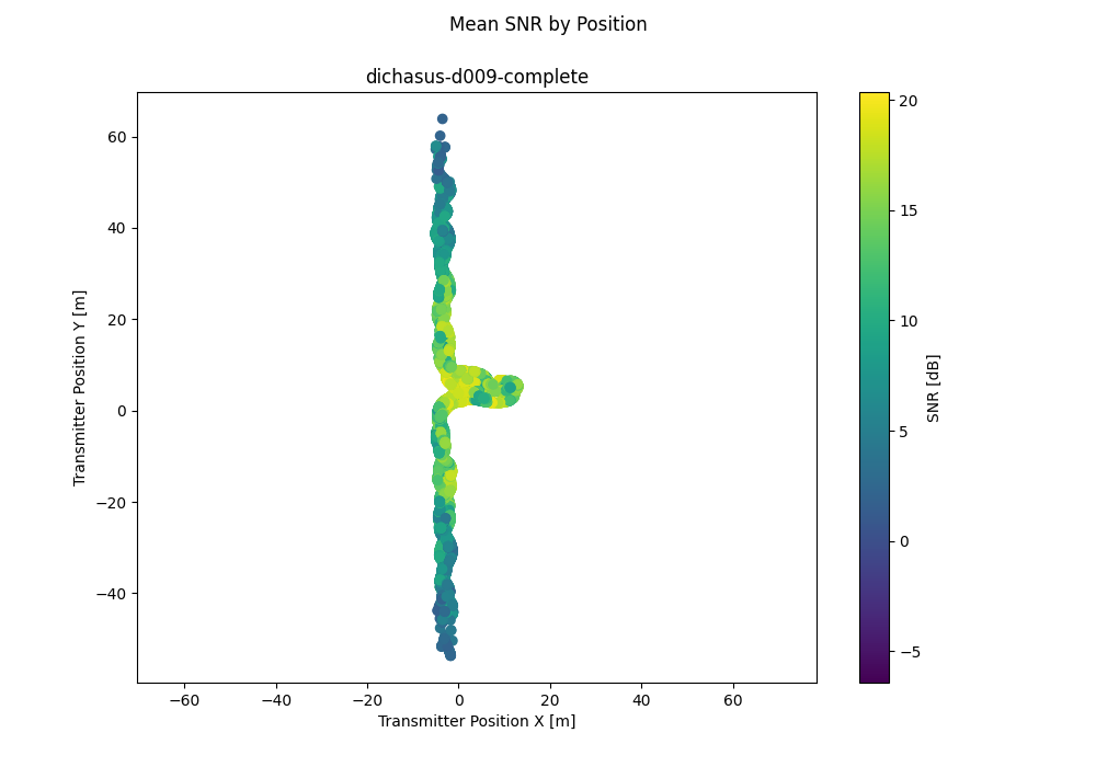
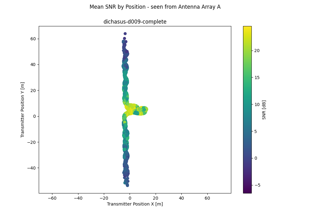
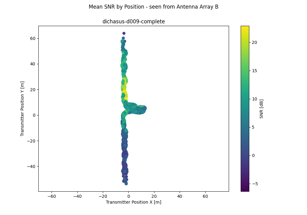
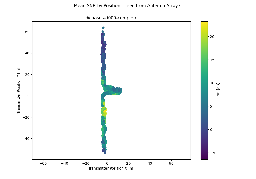
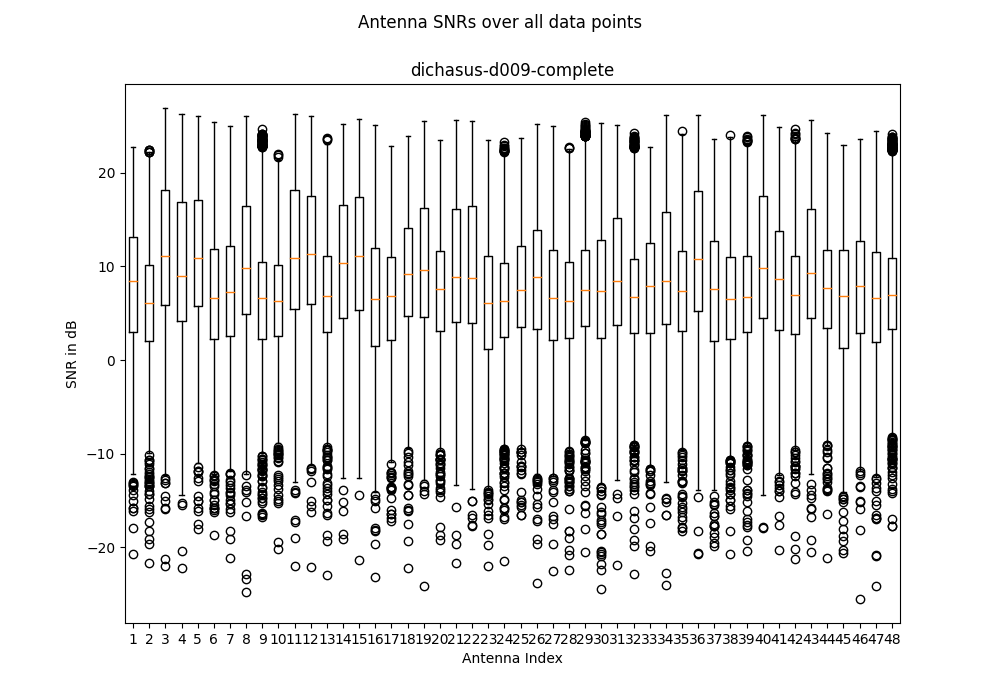
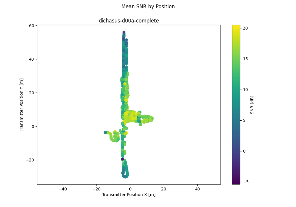
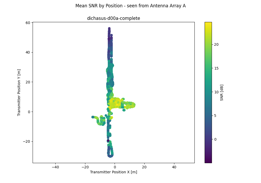
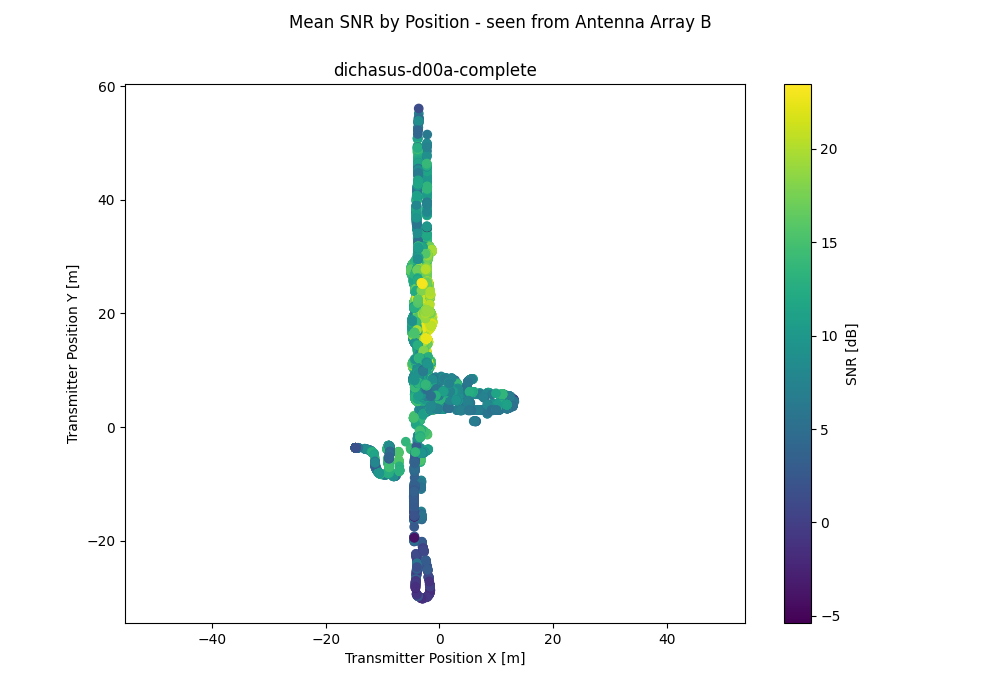
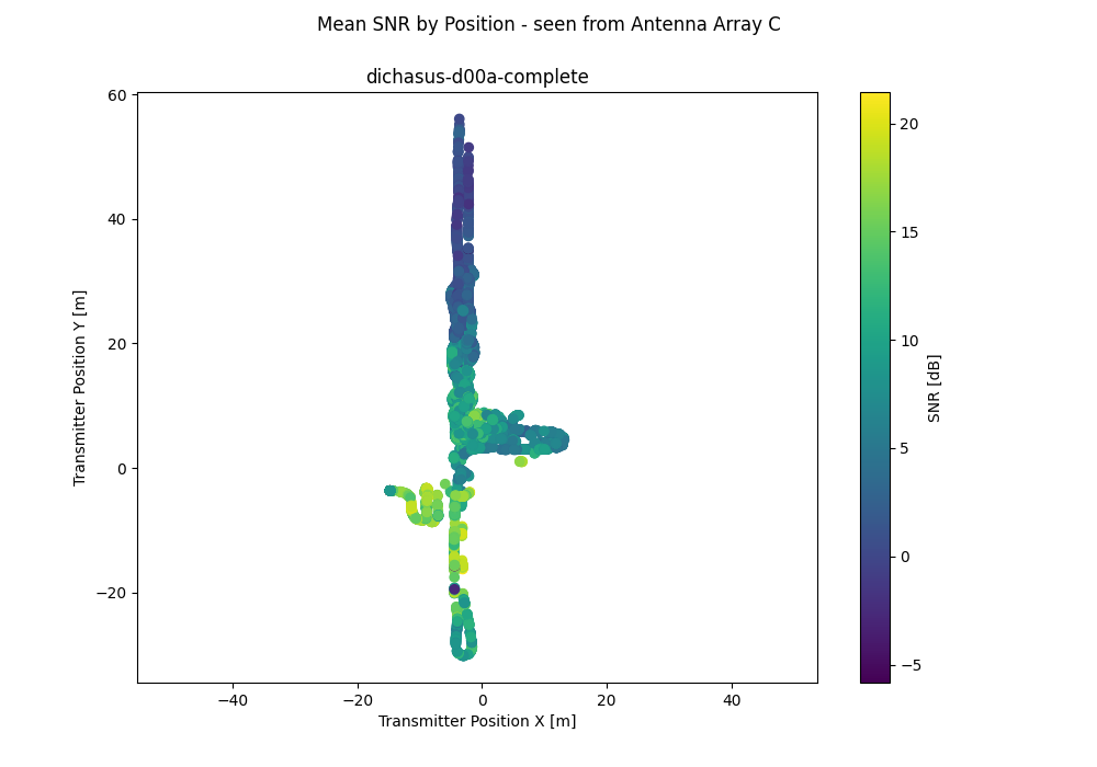
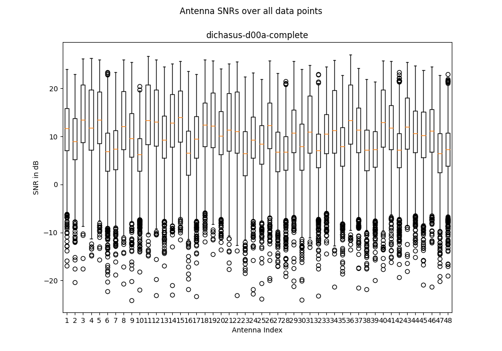
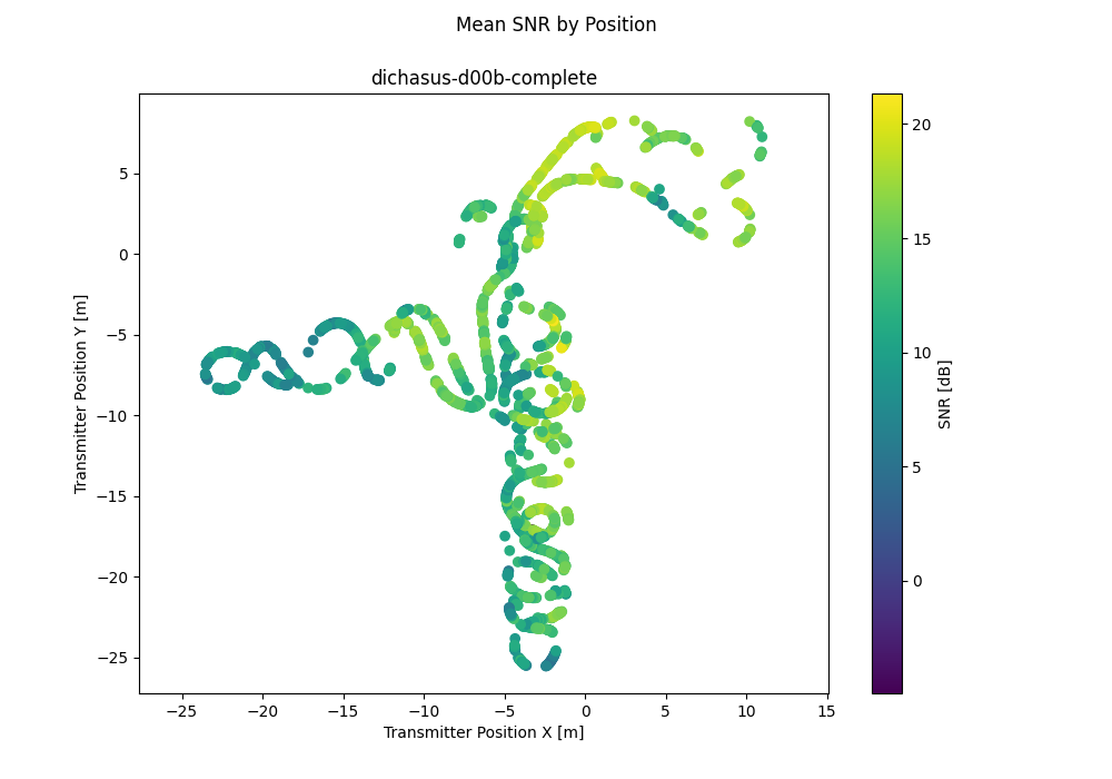
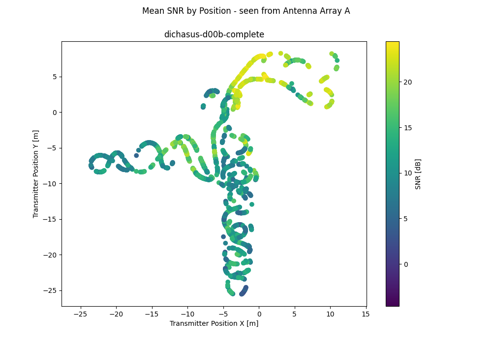
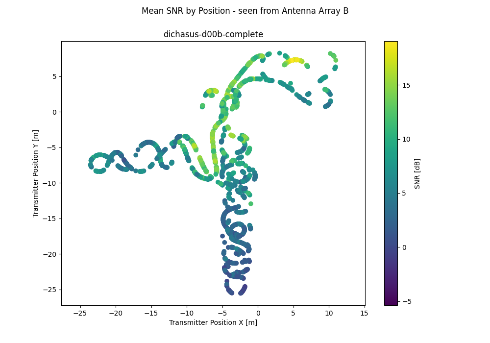
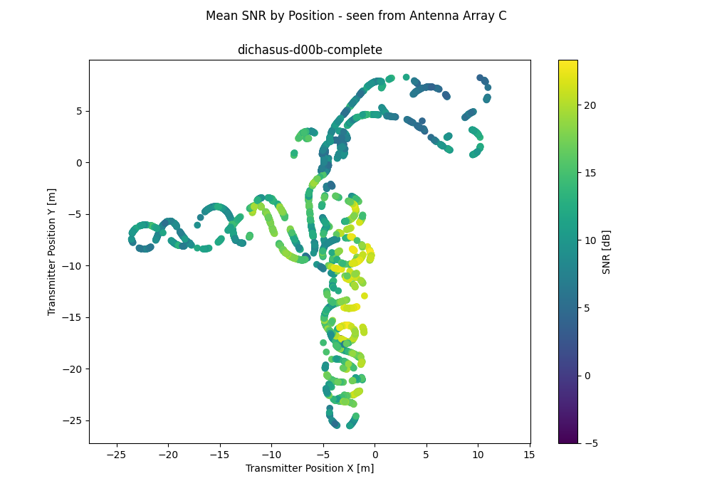
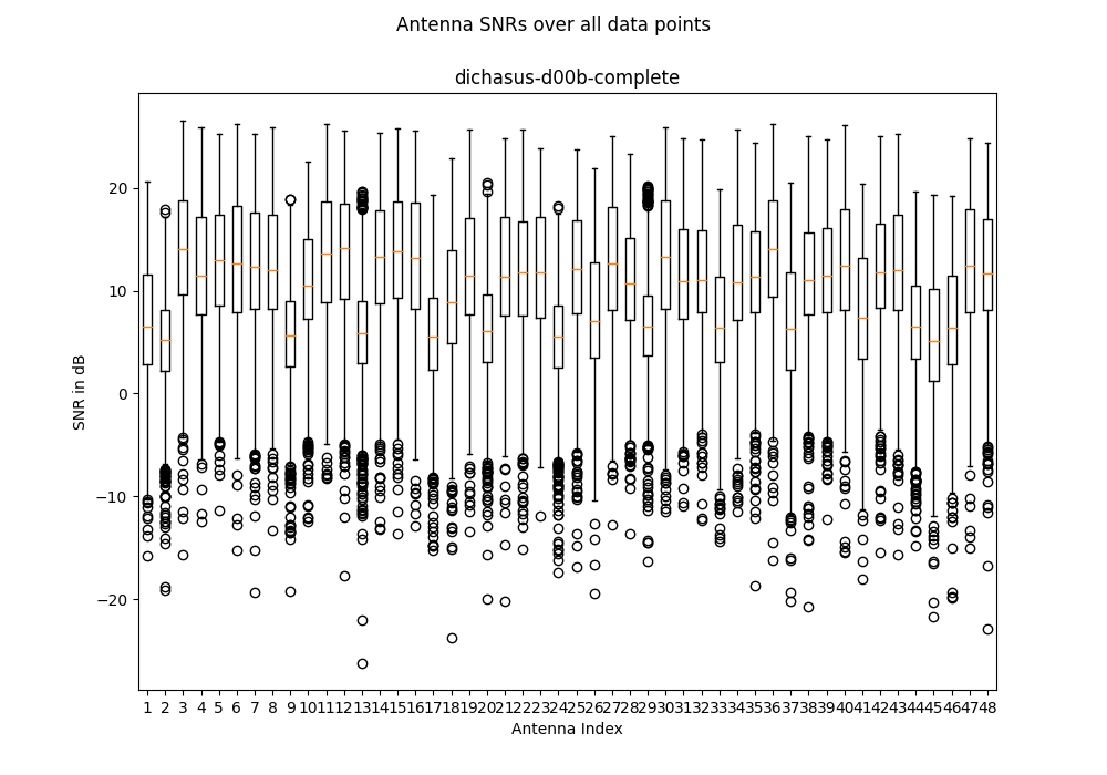
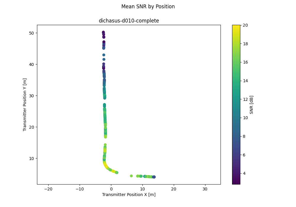
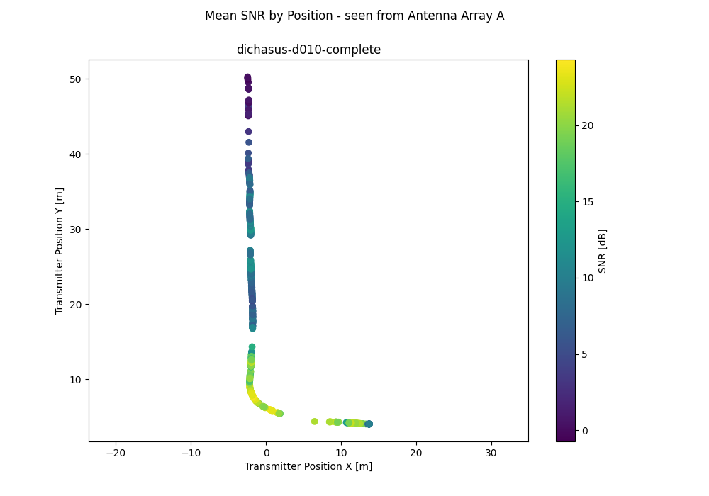
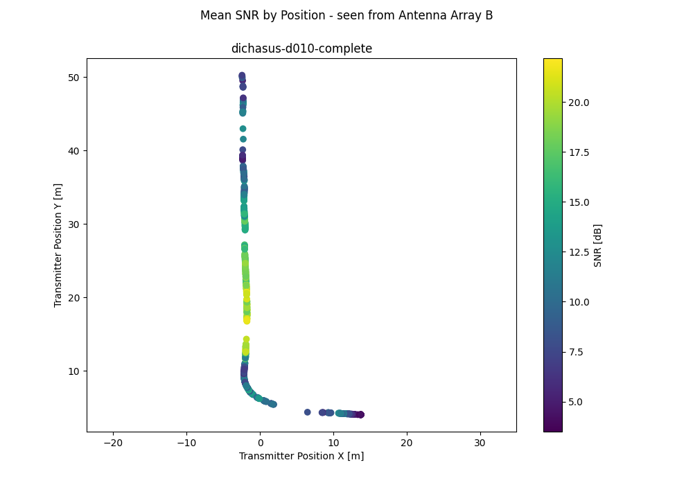
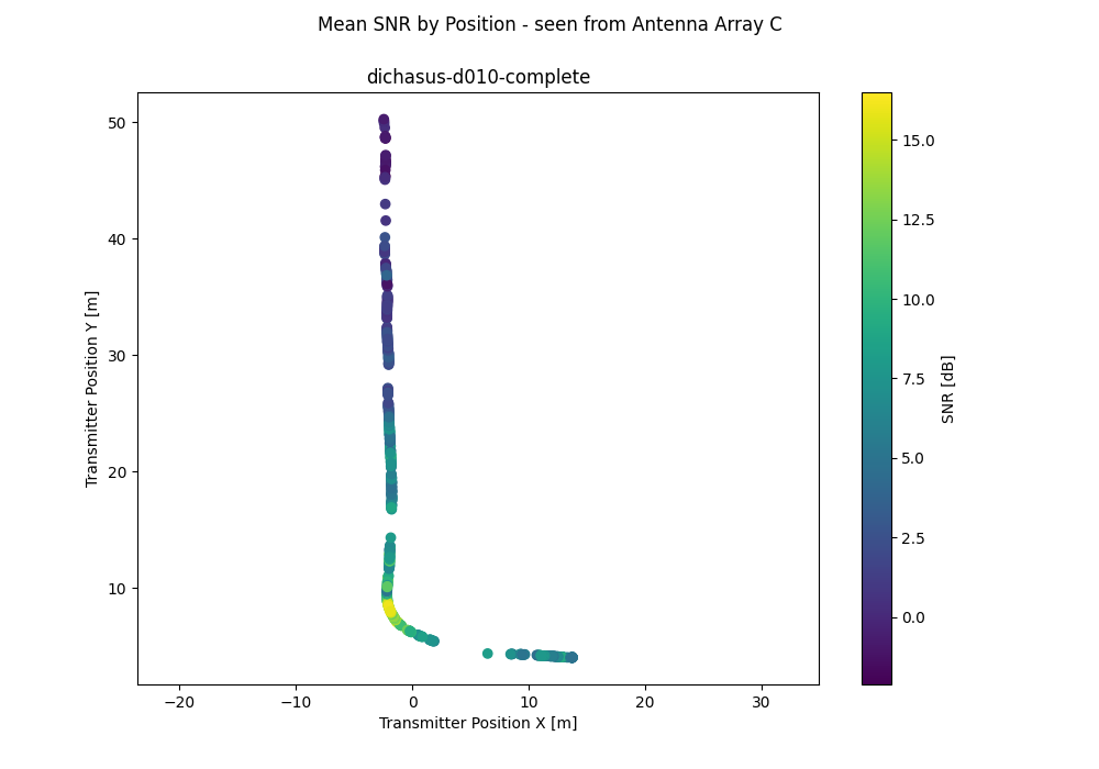
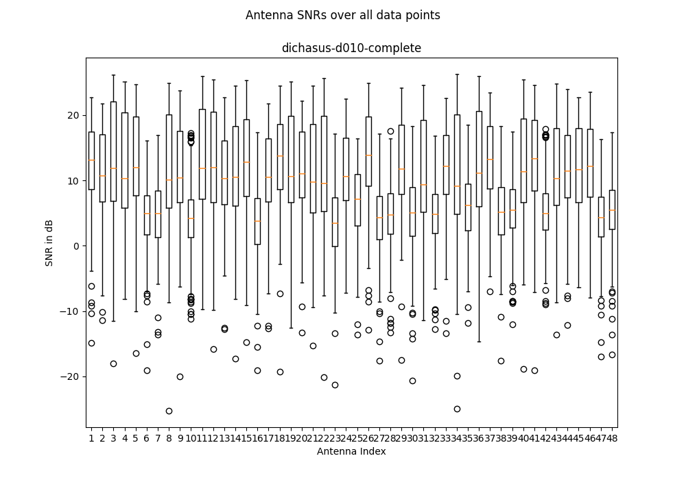
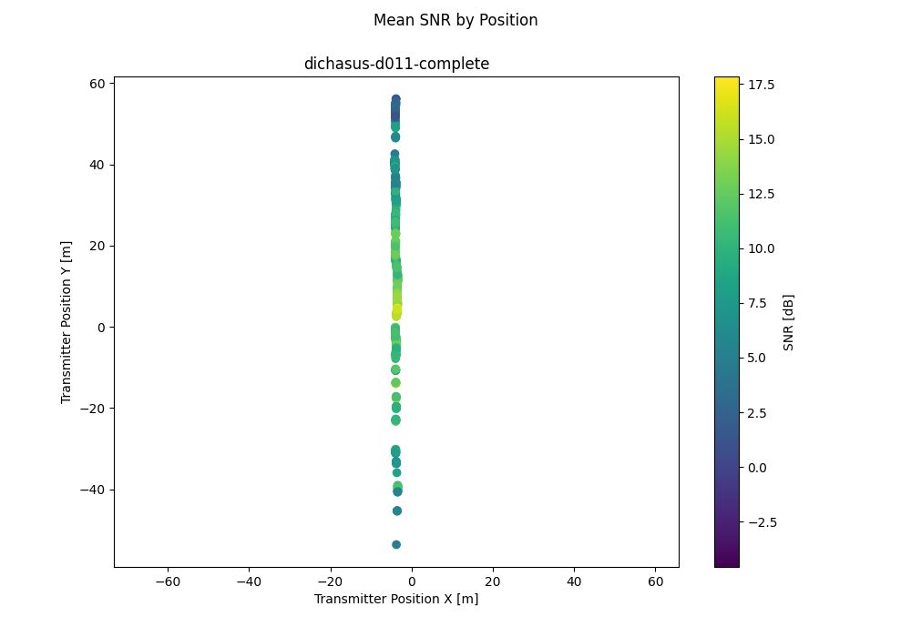
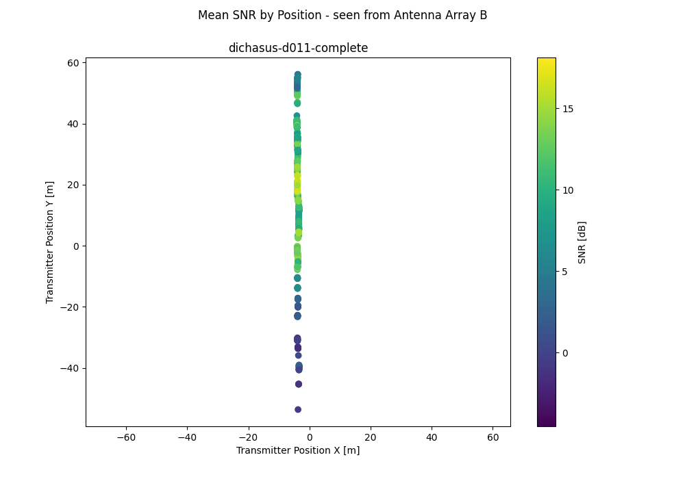
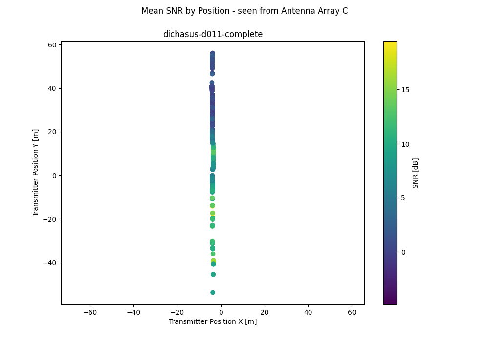
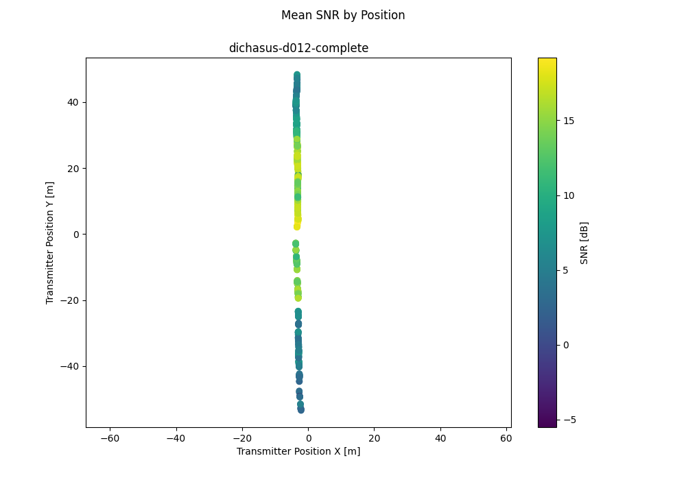
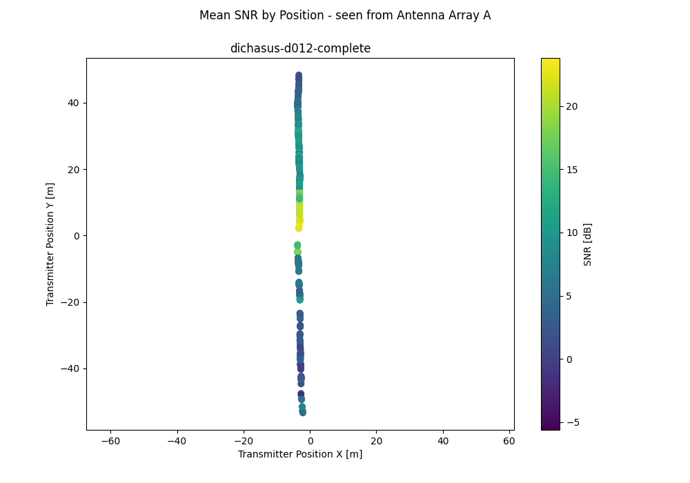
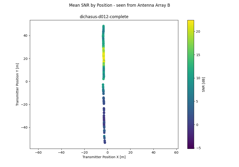
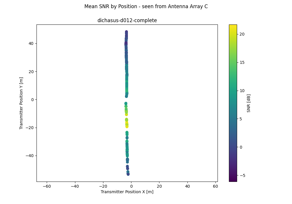
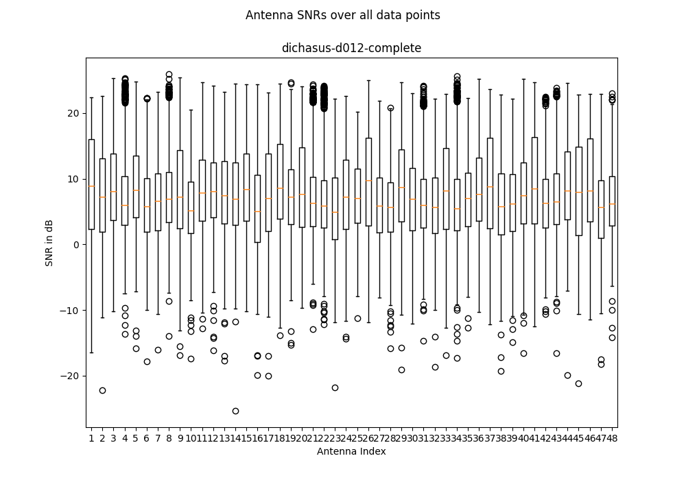
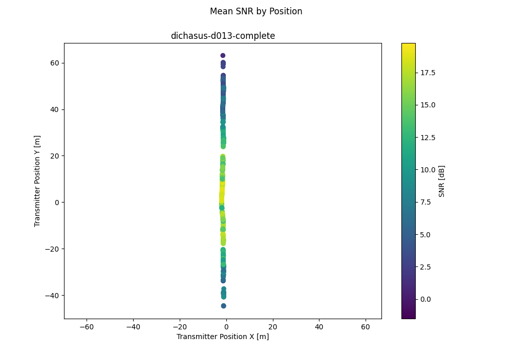
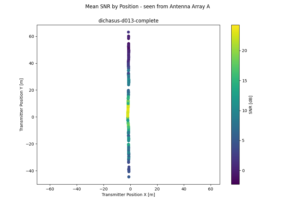
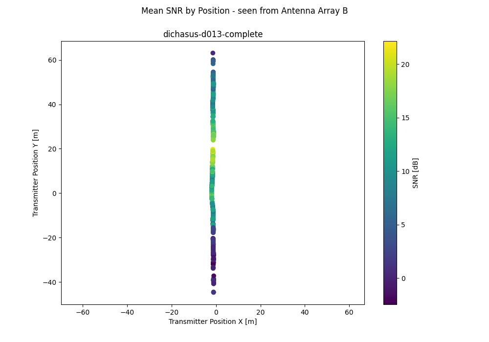
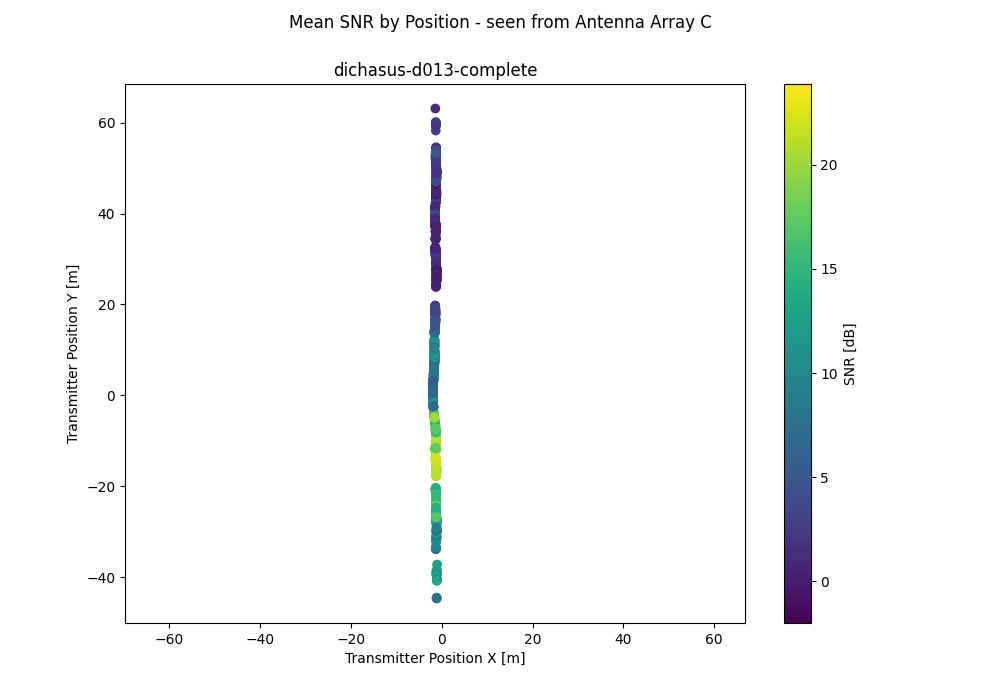
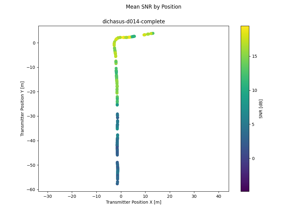
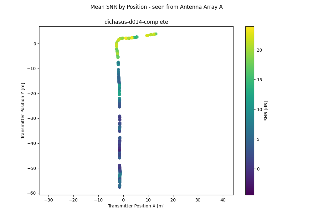
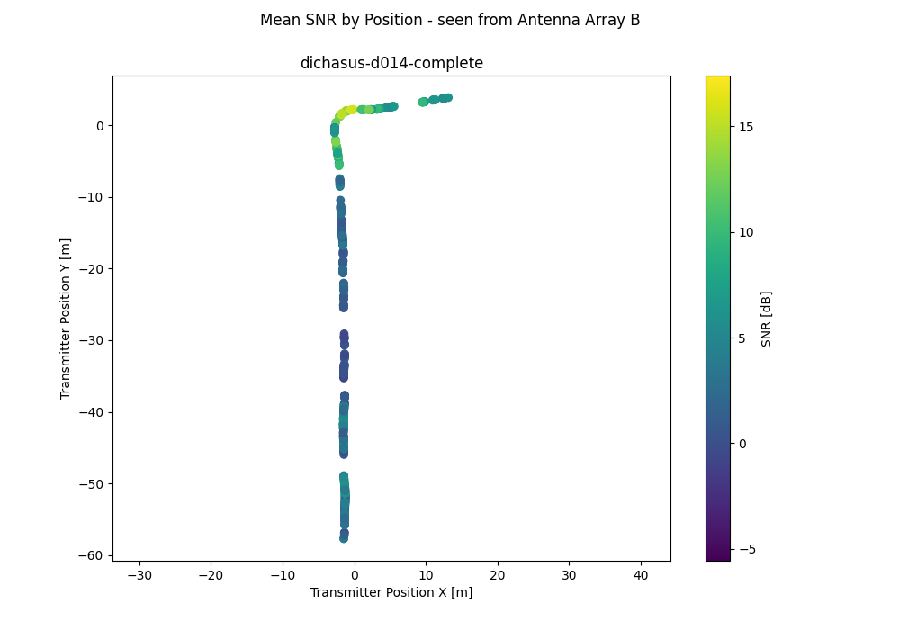
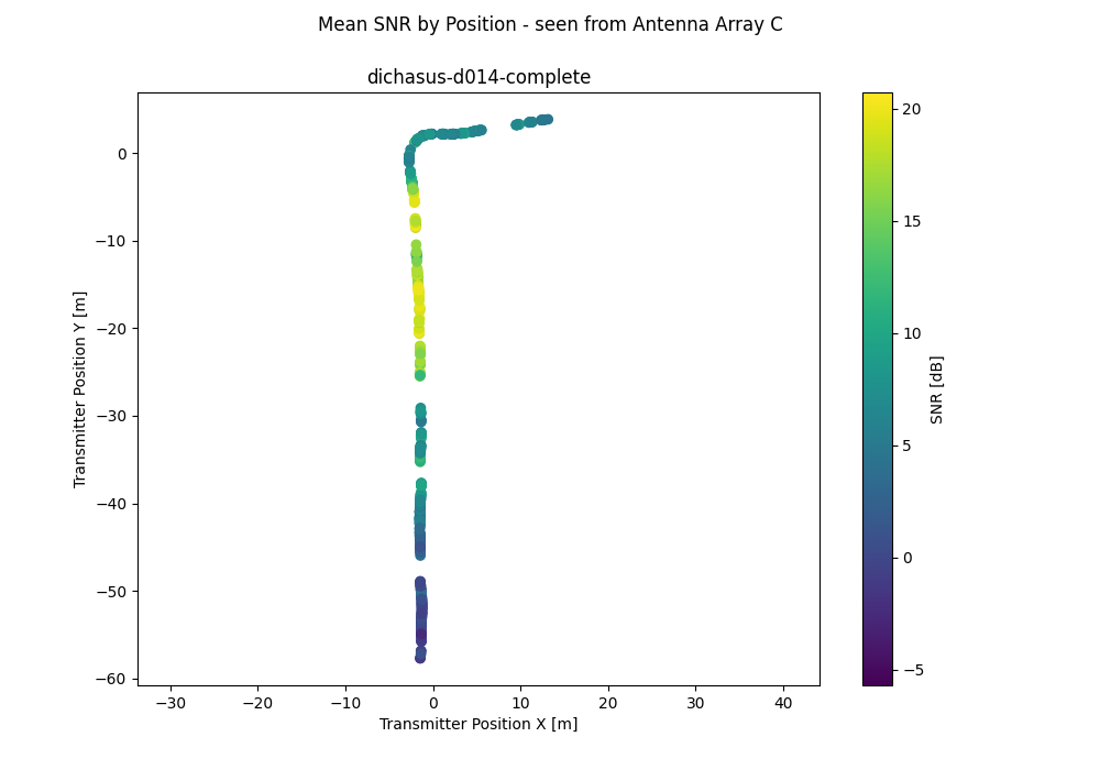
Three separate antenna arrays are attached to the facade of the Institute of Telecommunications building on the University of Stuttgart campus in Stuttgart-Vaihingen. The transmitter is mounted on a handcart and pulled around on the street in front of that building. The position of the tip of the transmit antenna is accurately tracked by a Tachymeter. This dataset only contains datapoints for which all 48 antennas have successfully acquired channel state information. Since one antenna in array B was not perfectly reliable due to synchronization issues, some datapoints might be missing (but all the contained datapoints should be accurate).
50.000 MHz
Signal Bandwidth
1024
OFDM Subcarriers
72709
Data Points
5972.0 s
Total Duration
28.6 GB
Total Download Size
48
Number of Antennas
Outdoor
Type of Environment
1.272000 GHz
Carrier Frequency
Distributed
Antenna Setup
3D Tachymeter
Position-Tagged
Experiment Setup
Data Analysis
Antenna Configuration
Antenna 1: Antenna Array A
| 4 | 13 | 39 | 14 | 2 | 35 | 10 | 11 |
| 42 | 33 | 30 | 18 | 7 | 20 | 3 | 21 |
Antenna 2: Antenna Array B
| 32 | 40 | 45 | 44 | 36 | 25 | 0 | 17 |
| 43 | 8 | 16 | 19 | 12 | 1 | 23 | 28 |
Antenna 3: Antenna Array C
| 24 | 5 | 26 | 22 | 15 | 46 | 29 | 6 |
| 47 | 9 | 41 | 27 | 34 | 37 | 31 | 38 |
Python: Import with TensorFlow
#!/usr/bin/env python3
import tensorflow as tf

raw_dataset = tf.data.TFRecordDataset(["tfrecords/dichasus-d002-complete.tfrecords", "tfrecords/dichasus-d004-complete.tfrecords", "tfrecords/dichasus-d005-complete.tfrecords", "tfrecords/dichasus-d006-complete.tfrecords", "tfrecords/dichasus-d007-complete.tfrecords", "tfrecords/dichasus-d008-complete.tfrecords", "tfrecords/dichasus-d009-complete.tfrecords", "tfrecords/dichasus-d00a-complete.tfrecords", "tfrecords/dichasus-d00b-complete.tfrecords", "tfrecords/dichasus-d010-complete.tfrecords", "tfrecords/dichasus-d011-complete.tfrecords", "tfrecords/dichasus-d012-complete.tfrecords", "tfrecords/dichasus-d013-complete.tfrecords", "tfrecords/dichasus-d014-complete.tfrecords"])

feature_description = {
	"cfo": tf.io.FixedLenFeature([], tf.string, default_value = ''),
	"csi": tf.io.FixedLenFeature([], tf.string, default_value = ''),
	"gt-interp-age-tachy": tf.io.FixedLenFeature([], tf.float32, default_value = 0),
	"pos-tachy": tf.io.FixedLenFeature([], tf.string, default_value = ''),
	"snr": tf.io.FixedLenFeature([], tf.string, default_value = ''),
	"time": tf.io.FixedLenFeature([], tf.float32, default_value = 0),
}

def record_parse_function(proto):
	record = tf.io.parse_single_example(proto, feature_description)

	# Measured carrier frequency offset between MOBTX and each receive antenna.
	cfo = tf.ensure_shape(tf.io.parse_tensor(record["cfo"], out_type = tf.float32), (48))

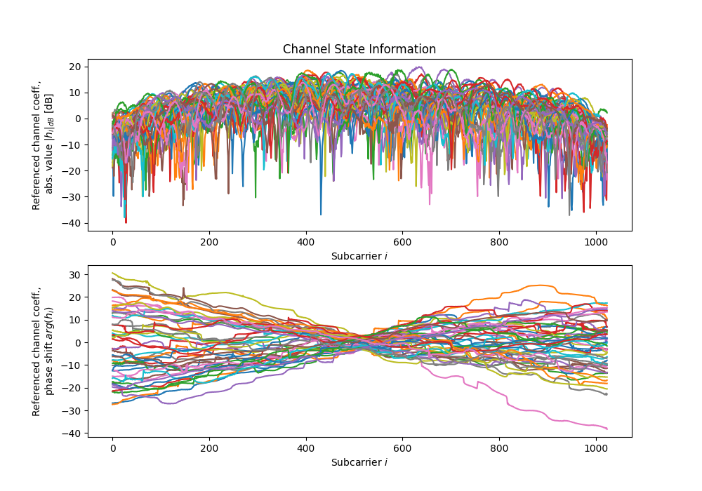
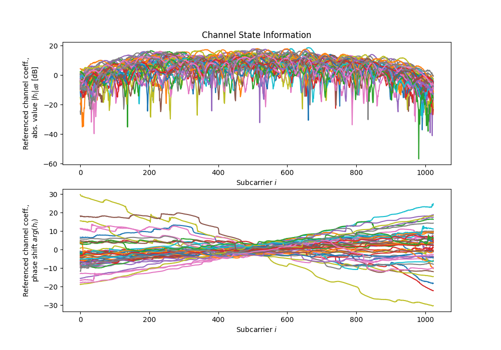
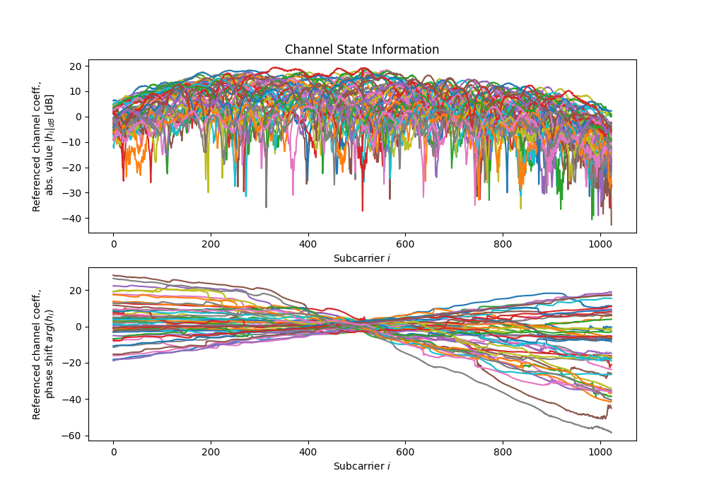
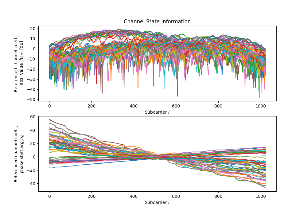
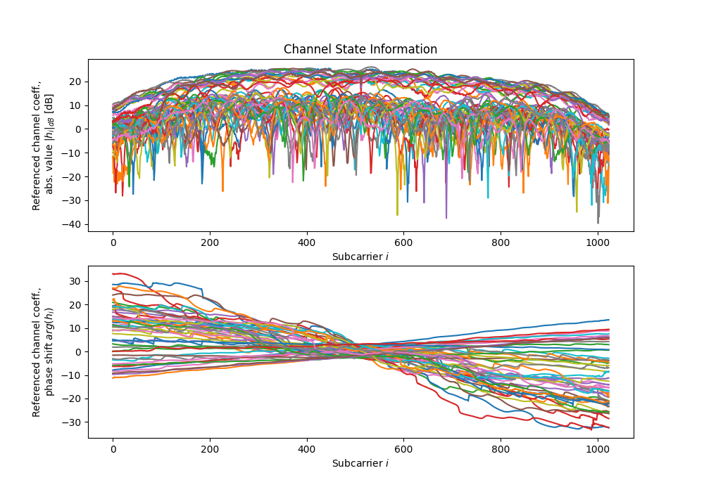
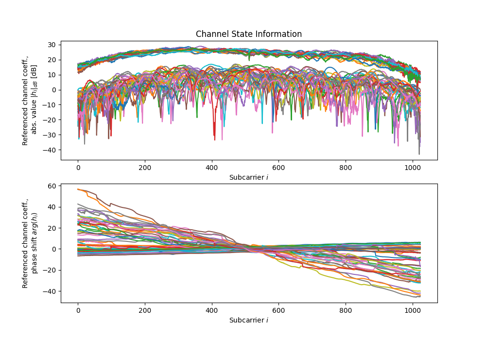
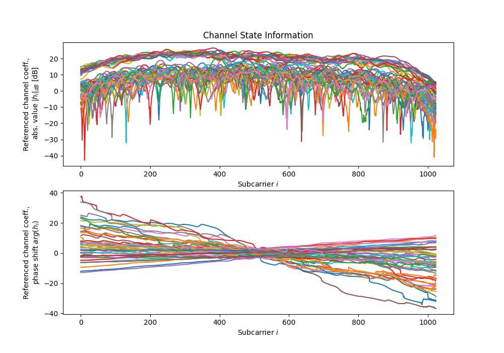
	# Channel coefficients for all antennas, over all subcarriers, real and imaginary parts
	csi = tf.ensure_shape(tf.io.parse_tensor(record["csi"], out_type = tf.float32), (48, 1024, 2))

	# Time in seconds to closest known tachymeter position. Indicates quality of linear interpolation.
	gt_interp_age_tachy = tf.ensure_shape(record["gt-interp-age-tachy"], ())

	# Position of transmitter determined by a tachymeter pointed at a prism mounted on top of the antenna, in meters (X / Y / Z coordinates)
	pos_tachy = tf.ensure_shape(tf.io.parse_tensor(record["pos-tachy"], out_type = tf.float64), (3))

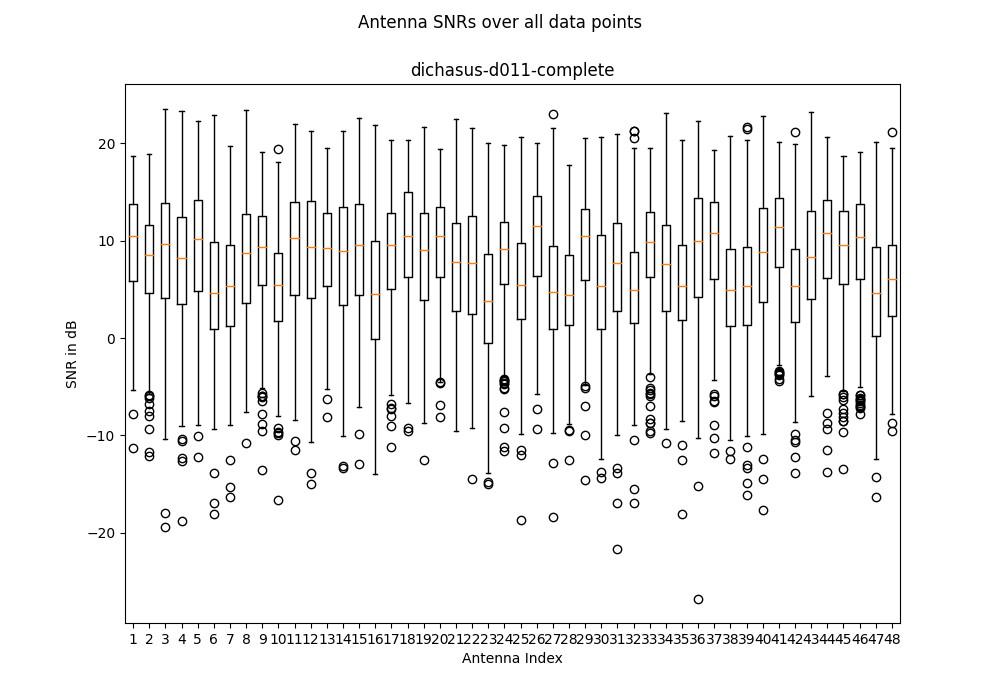
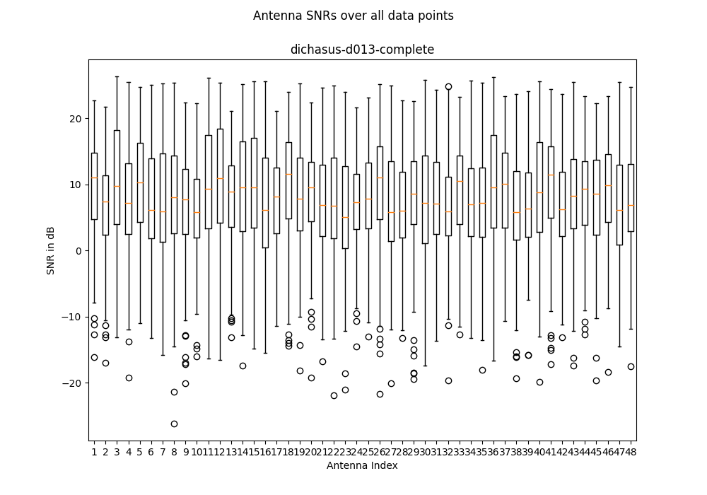
	# Signal-to-Noise ratio estimates for all antennas
	snr = tf.ensure_shape(tf.io.parse_tensor(record["snr"], out_type = tf.float32), (48))

	# Timestamp since start of measurement campaign, in seconds
	time = tf.ensure_shape(record["time"], ())

	return cfo, csi, gt_interp_age_tachy, pos_tachy, snr, time

dataset = raw_dataset.map(record_parse_function, num_parallel_calls = tf.data.experimental.AUTOTUNE)

# Optional: Cache dataset in RAM for faster training
dataset = dataset.cache()
Reference Channel Compensation
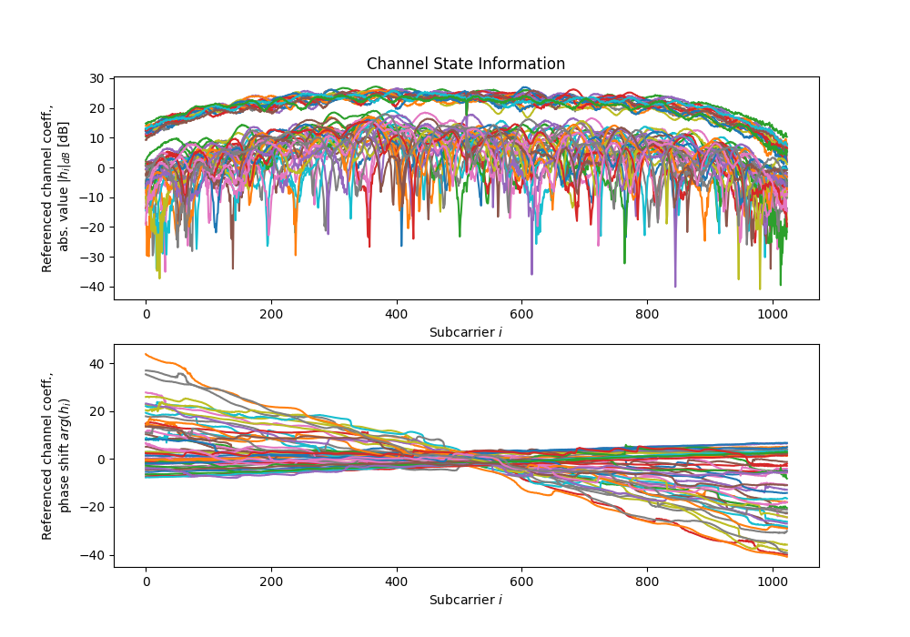
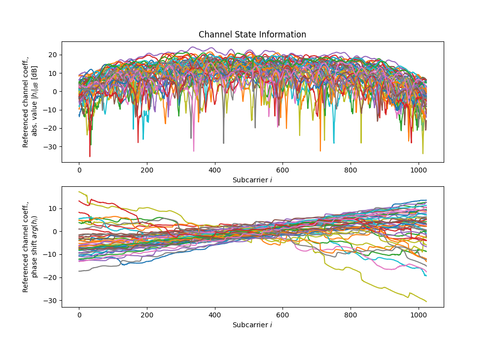
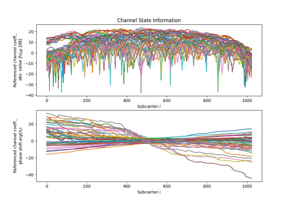
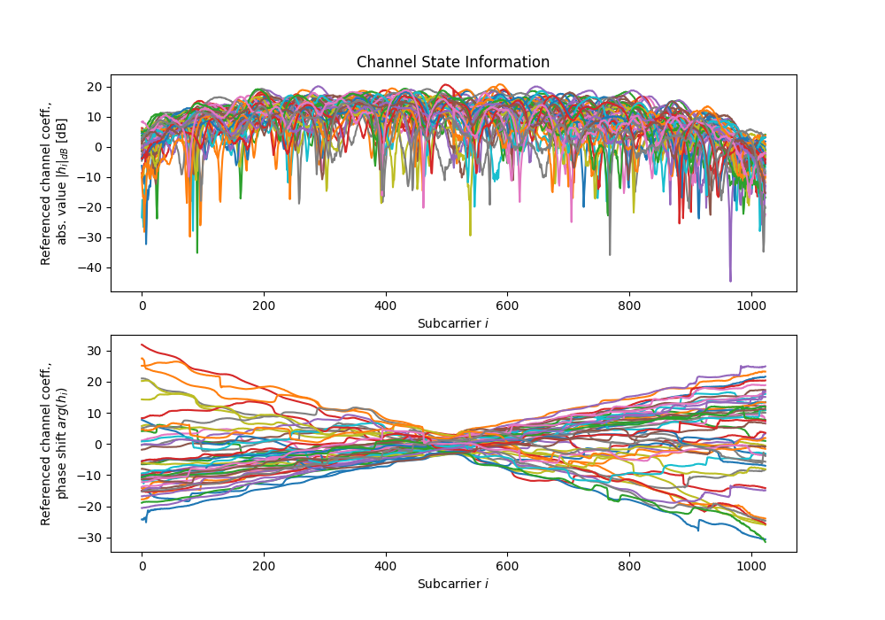
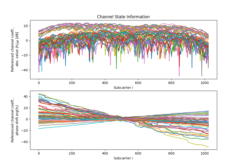
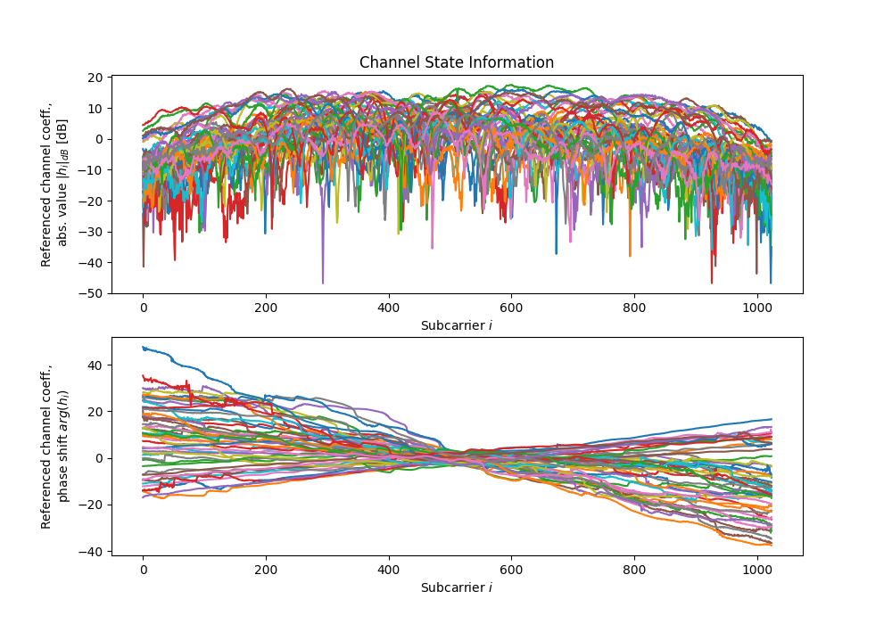
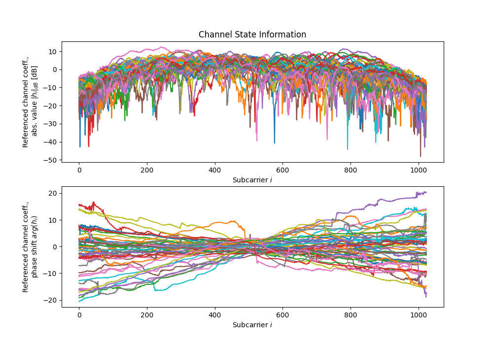
For this dataset, we are able to provide estimated antenna-specific carrier phase and sampling time offsets. These offsets occur due to the fact that the reference transmitter channel is not perfectly frequency-flat. To learn more about why these offsets occur and about their compensation, visit our offset calibration tutorial on this topic. Note that the estimates provided here are "best-effort" calculations. The phase and time offsets between antennas in the same array are usually very accurate, but for antennas that are spaced far apart, the results may be less precise. The offset are constant over the complete dataset.How to Cite
Please refer to the home page for information on how to cite any of our datasets in your research. For this dataset in particular, you may use the following BibTeX:
@data{dataset-dichasus-dxxx-complete,
	author    = {Euchner, Florian and Gauger, Marc},
	publisher = {DaRUS},
	title     = {{CSI Dataset dichasus-dxxx-complete: Outdoor - Three arrays distributed along the facade}},
	doi       = {doi:10.18419/darus-3153},
	url       = {https://doi.org/doi:10.18419/darus-3153},
	year      = {2022}
}
Download
This dataset consists of 14 files. Descriptions of these files as well as download links are provided below.
dichasus-d002-complete
dichasus-d004-complete
dichasus-d005-complete
dichasus-d006-complete
dichasus-d007-complete
dichasus-d008-complete
dichasus-d009-complete
dichasus-d00a-complete
dichasus-d00b-complete
dichasus-d010-complete
dichasus-d011-complete
dichasus-d012-complete
dichasus-d013-complete
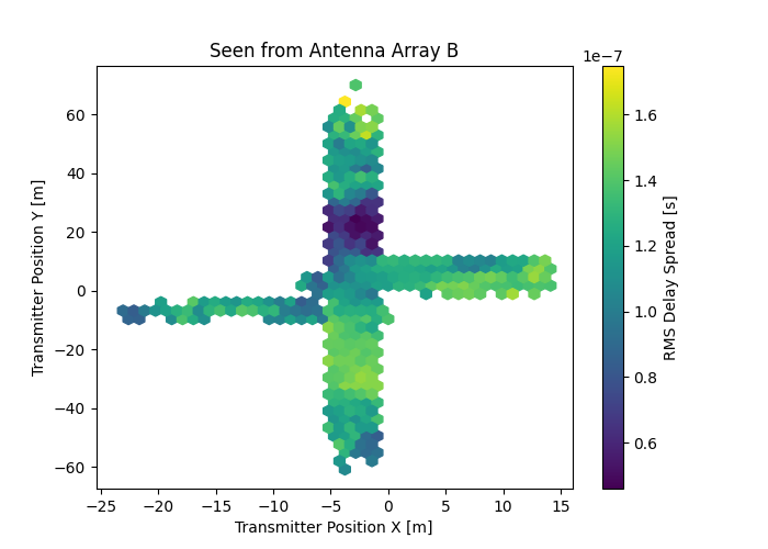
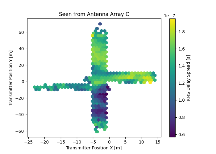
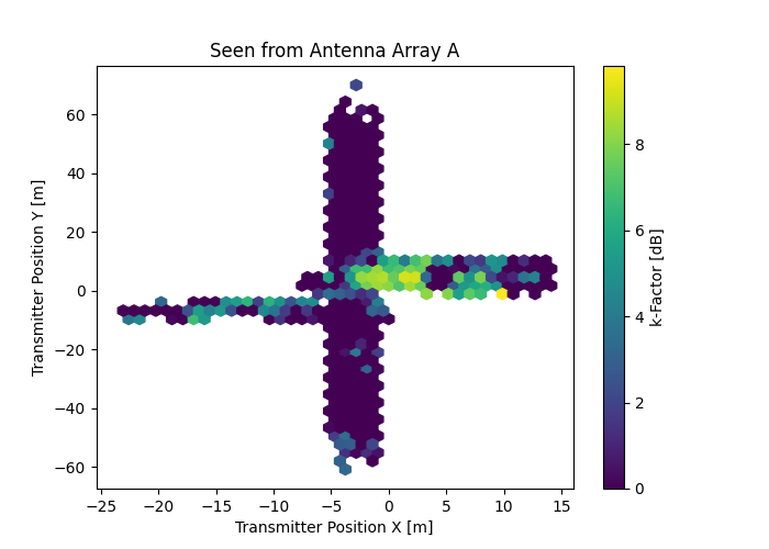
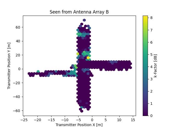
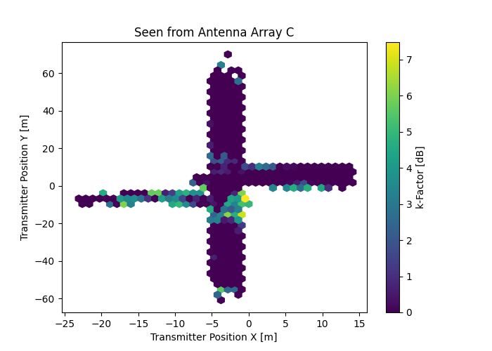
Derived Channel Statistics
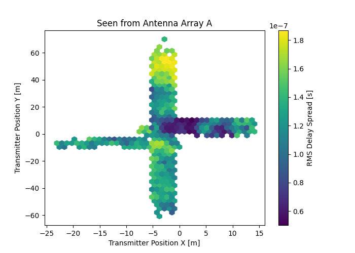
Channel statistics such as delay spread, k-Factor and path loss exponent are a good way to characterize a wireless channel measurement and to parametrize a channel model. Using estimation algorithms contributed by Janina Sanzi, we automatically extract the following channel statistics from the measured datasets:

