Compensating for the Reference Transmitter Channel

What are static phase offsets?

In this tutorial, we will try to visualize the received phases of the receive antennas and apply a classical AoA estimation method to a DICHASUS dataset. We will see that before we can do any of this, we need to compensate for the constant receiver-specific carrier phase offsets (CPOs) and sampling time offsets (STOs).

But wait: Isn't it strange that there are any phase and time offsets in the first place? Looking at an overview of the system architecture, you can see that the antenna array receivers (AARX) should be able to receive both the reference transmitter (REFTX) for synchronization and mobile "main" transmitter (MOBTX) for channel measurements. Isn't the whole purpose of the over-the-air synchronization in DICHASUS to make all receivers coherent in frequency, time and also in phase?

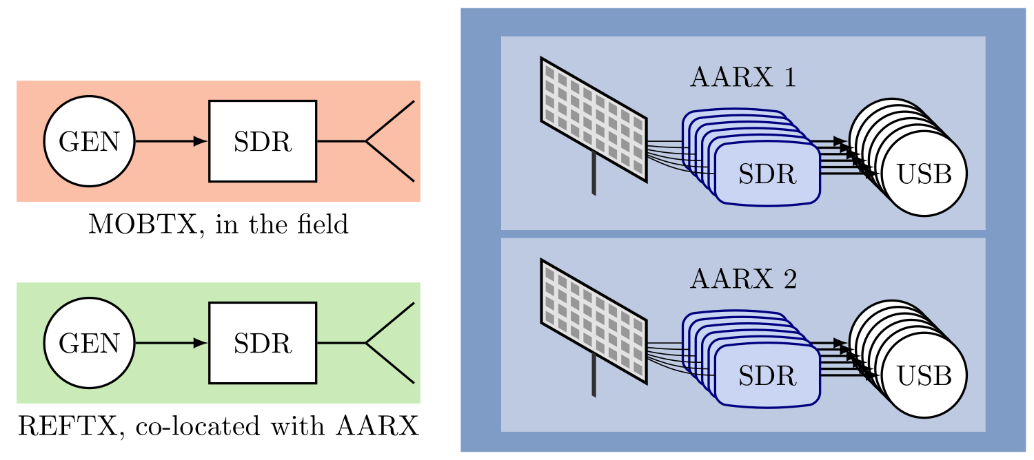
Well, it's true that all receivers (AARX) are synchronous to the reference signal, also called synchronization broadcast. However, they can only be synchronous to their respective received synchronization signal, not to the one that was actually transmitted. In other words, the channel between the reference transmitter (REFTX) and each receiver (AARX) has an impact on the synchronization!

While almost all receivers should have a good (line-of-sight or, at least, low-attenuation) channel to the REFTX, each REFTX-receiver path may experience a different phase shift and path delay. This is because the REFTX signal still has to pass through a real-world physical environment channel, with different path lengths and possibly even multipath propagation.

Without Offset Compensation

For now, we are going to completely ignore the issue of static phase offsets. Let's find out what happens if we plot the received phases over the physical position of antennas in the antenna array without any prior calibration whatsoever. In a line-of-sight scenario, we should, assuming phase-coherent receivers, hopefully see some patterns emerge, depending on the location of the transmitter. In this tutorial, we will use a single robot round trip from the dichasus-015x dataset, namely dichasus-0152:

!mkdir dichasus
!wget --content-disposition https://darus.uni-stuttgart.de/api/access/datafile/:persistentId?persistentId=doi:10.18419/darus-2202/2 -P dichasus # dichasus-0152

import matplotlib.colors as colors
import matplotlib.pyplot as plt
import matplotlib.cm as cm
import tensorflow as tf
import numpy as np
import json
%matplotlib inline

def record_parse_function(proto):
	record = tf.io.parse_single_example(proto, {
		"csi": tf.io.FixedLenFeature([], tf.string, default_value = ''),
		"pos-tachy": tf.io.FixedLenFeature([], tf.string, default_value = '')
	})
		
	csi = tf.io.parse_tensor(record["csi"], out_type = tf.float32)
	csi = tf.signal.fftshift(csi, axes = 1)
	csi = tf.complex(csi[:,:,0], csi[:,:,1])
	pos_tachy = tf.ensure_shape(tf.io.parse_tensor(record["pos-tachy"], out_type = tf.float64), (3))
		
	# We only care about x/y position dimensions, z is always close to 0
	return csi, pos_tachy[:2]
	
datafiles = ["dichasus/dichasus-0152.tfrecords"]
dataset = tf.data.TFRecordDataset(datafiles).map(record_parse_function)
dataset = dataset.cache()

Our goal is to plot the received signal phases over the physical antenna position. Obviously, these phases depend on the transmitter position. We could, in theory, just create a plot for each and every datapoint in the whole dataset - for this tutorial, we will concentrate on three different, representative transmitter locations though:

• Frontal: The transmitter is directly in front of the receiver antenna array, at a distance of 3m
• Left: Relative to the "frontal" position, the transmitter is moved 1m to the left of the antenna array
• Right: Relative to the "frontal" position, the transmitter is moved 1m to the right of the antenna array

# Generate filter function that returns true if datapoint was measured somewhere around given target location
def filter_around_point(point, radius):
	def f(csi, pos):
		return tf.norm(pos - tf.constant(point, dtype = tf.float64)) < radius
	return f
				
# Pass dataset through filter to generate frontal / left / right samples
points_frontal = dataset.filter(filter_around_point((-3.0, 0.0), 0.15))
points_left = dataset.filter(filter_around_point((-3.0, 1.0), 0.15))
points_right = dataset.filter(filter_around_point((-3.0, -1.0), 0.15))

To do that, though, we first have to figure out where to draw the measured phases, i.e., how to assign each of the phase values to an antenna in the array. All the required information for this is given at the dataset's description page, namely in the antenna configuration section.

Most importantly, this is where you will find the "channel assignments" table. This table contains the mapping from the channel of the CSI vector (i.e., its antenna index in the CSI tensor, here in the range 0-31) to the position of the antenna in the array, as seen from a viewpoint in front of the array. For dichasus-015x, these assignments are also illustrated in the picture. Please note that the assignments may be different from one dataset to another!

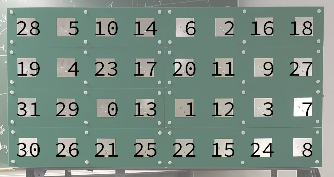
assignments = [
	[28,5,10,14,6,2,16,18],
	[19,4,23,17,20,11,9,27],
	[31,29,0,13,1,12,3,7],
	[30,26,21,25,22,15,24,8]
]
			
antennacount = np.sum([len(line) for line in assignments])
antennapos = np.zeros((antennacount, 2), dtype = int)
			
for y in range(len(assignments)):
	for x in range(len(assignments[y])):
		antennapos[assignments[y][x]] = np.asarray((x, y))

Furthermore, the function still takes a TensorFlow dataset as an input (its first parameter). This dataset should already be filtered down to only contain datapoints within a limited physical area, as the function will average the received phases also over all contained datapoints.

def plot_array_phases(dataset, subcarrier_start, subcarrier_count, title):
	dataset_phases = []
	
	for csi, pos in dataset:
		datapoint_phases = np.sum(csi.numpy()[:, subcarrier_start:subcarrier_start + subcarrier_count], axis = 1)
		datapoint_phases = datapoint_phases * np.conj(datapoint_phases[0])
		dataset_phases.append(datapoint_phases)
	
	antenna_phases_frontview = np.zeros((len(assignments), len(assignments[0])), dtype = np.complex128)
	for antenna, phase in enumerate(np.sum(dataset_phases, axis = 0)):
		pos = antennapos[antenna]
		antenna_phases_frontview[pos[1], pos[0]] = phase
	
	plt.title(title)
	plt.xlabel("Antenna Position X")
	plt.ylabel("Antenna Position Y")
	plt.imshow(np.angle(antenna_phases_frontview), cmap = plt.get_cmap("twilight"))
	plt.colorbar(shrink = 0.7)
	plt.show()

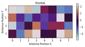
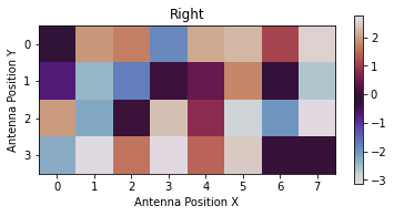
It is now time for the long-awaited moment of truth:

plot_array_phases(points_frontal, 512, 8, "Frontal")
plot_array_phases(points_left, 512, 8, "Left")
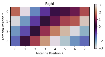
plot_array_phases(points_right, 512, 8, "Right")

The results we obtain are rather... disappointing. To put it bluntly, the phases we measure appear to be completely random, there is no visible pattern whatsoever. Even worse, just looking at the phase plots, there is no way on earth we would be able to distinguish the three different transmitter positions.

Admittedly, this is not really unexpected: We already established that each antenna has a constant phase and time offset that we have not compensated for up until this point. The seemingly random phase plots only illustrate this point once again.

So, how exactly do the phase and time offsets manifest themselves in the measured channel coefficients? To understand this, we must first recap some basics about channel coefficients, modulation and fourier transforms.

Phase and Timing Offset Compensation

As discussed earlier, while every receiver is synchronous to its received reference signal, this received signal may exhibit a receiver-specific, constant phase offset and time delay. The DICHASUS "main" transmitter (MOBTX) is based on a cyclic prefix-orthogonal frequency division multiplex (CP-OFDM) modulation. So, what happens if we demodulate the pilot symbols in the received MOBTX signal with a fixed phase and time offset? What is the effect of these time-domain shifts on the frequency-domain constellation symbols?

From Fourier analysis, we know that a shift of any signal \( s(t) \) in the time domain by \( \tau_\mathrm{STO} \) results in a multiplication with \( \mathrm e^{\mathrm j 2 \pi f \tau_\mathrm{STO} } \) in the frequency domain: \[ \mathcal F \left\{ s(t) \right\} = S(f) ~ \implies ~ \mathcal F \left\{ s(t - \tau_\mathrm{STO}) \right\} = S(f) \cdot \mathrm e^{\mathrm j 2 \pi \tau_\mathrm{STO} f} \] This is exactly what we experience when we demodulate an OFDM symbol without getting the sampling instances exactly right, but shifted by a constant delay. More specifically, if the "true" channel coefficient (just the physical environment phase shift, without offset) for the \( m \)-th receive antenna and the \( i \)-th subcarrier is given by \( h_{m, i} \), the channel coefficient that we actually measure is \[ a_{m, i} = h_{m, i} ~ \mathrm{e}^{\mathrm{j} (\varphi_m + 2 \pi ~ \tau_{\mathrm{STO}, m} ~ i \Delta f_\mathrm{sub, mob})}. \] In this equation, \( \varphi_m \) denotes the static phase offset term for antenna \( m \), \( \tau_{\mathrm{STO}, m} \) is its sampling time offset and \( \Delta f_\mathrm{sub, mob} \) is the subcarrier spacing. Here, \( \tau_{\mathrm{STO}, m} \) is expressed in a physical unit of time, i.e., in seconds. For practical purposes, it can be a advantageous to normalize \( \tau_{\mathrm{STO}, m} \) to the sampling interval \( t_\mathrm{s} = \frac{1}{B} \) (with signal bandwidth = sampling frequency \( B \)) to obtain a sampling time offset \( d_{\mathrm{STO}, m} = B ~ \tau_{\mathrm{STO}, m} \) value measured in samples. In addition, we can also rewrite \( \Delta f_\mathrm{sub, mob} \) as \( \Delta f_\mathrm{sub, mob} = \frac{B}{N_\mathrm{sub}} \), where \( N_\mathrm{sub} \) denotes the total number of subcarriers. With these simplifications, we finally obtain \[ a_{m, i} = h_{m, i} ~ \mathrm{e}^{\mathrm{j} \left(\varphi_m + 2 \pi ~ d_{\mathrm{STO}, m} ~ \frac{i}{N_\mathrm{sub}}\right)}. \]

The above equation contains a phase correction term \( \mathrm{e}^{\mathrm{j} \left(\varphi_m + 2 \pi ~ d_{\mathrm{STO}, m} ~ \frac{i}{N_\mathrm{sub}}\right)} \) for every subcarrier channel coefficient. For any channel coefficient with antenna index \( m \) and the subcarrier index \( i \), this correction term can be computed based on \( \varphi_m \) and \( d_{\mathrm{STO}, m} \). Luckily, we at the Institute of Telecommunications have found a reliable method to estimate these two offset parameters and we are publishing our calibration data alongside every applicable dataset. For dichasus-015x, you can download a JSON file with these parameters from our website:

# Download JSON file with phase offsets (in radians) and sampling time offsets (in samples)
!wget https://dichasus.inue.uni-stuttgart.de/datasets/data/dichasus-015x/reftx-offsets-dichasus-015x.json -P dichasus

offsets = None

with open("dichasus/reftx-offsets-dichasus-015x.json", "r") as offsetfile:
	offsets = json.load(offsetfile)

{
	"cpo" : [ list of carrier phase offsets in radians, for antennas 0...31 ],
	"sto" : [ list of sampling time offsets in samples, for antennas 0...31 ]
}

Let's plot the phase of the phase correction term, namely \( \varphi_m + 2 \pi ~ d_{\mathrm{STO}, m} ~ \frac{i}{N_\mathrm{sub}} \), for all 32 antennas (different colors) over all subcarrier indices \( i \):

sto_offset = tf.tensordot(tf.constant(offsets["sto"]), 2 * np.pi * tf.range(1024, dtype = np.float32) / 1024.0, axes = 0)
cpo_offset = tf.tensordot(tf.constant(offsets["cpo"]), tf.ones(1024, dtype = np.float32), axes = 0)
correction_phase = (sto_offset + cpo_offset).numpy()
plt.figure(figsize=(8, 5))
plt.xlabel("Subcarrier Index")
plt.ylabel("Phase Correction Term [rad]")
plt.plot(np.transpose(correction_phase))
plt.show()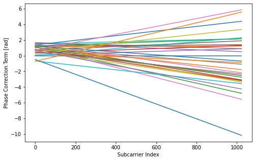

Nothing surprising here, really. Clearly, the phase offset leads to a subcarrier-specific phase shift that increases linearly over the subcarrier index. For this particular dataset, the antenna corresponding to the blue curve (antenna number 30) has the largest time offset, \( d_\mathrm{STO, 30} \approx -1.5 \) samples.

Once we know how to compute the constant phase correction terms for all channel coefficients, it is easy to calibrate of datapoints. We do this by writing a a map function that can be applied to each element (CSI tensor and label) of the dataset to calibrate. The function is written such that it is independent of the number of subcarriers used to measure the particular dataset.

def apply_calibration(csi, pos):
	sto_offset = tf.tensordot(tf.constant(offsets["sto"]), 2 * np.pi * tf.range(tf.shape(csi)[1], dtype = np.float32) / tf.cast(tf.shape(csi)[1], np.float32), axes = 0)
	cpo_offset = tf.tensordot(tf.constant(offsets["cpo"]), tf.ones(tf.shape(csi)[1], dtype = np.float32), axes = 0)
	csi = tf.multiply(csi, tf.exp(tf.complex(0.0, sto_offset + cpo_offset)))
	return csi, pos

Let's test the calibration function on our three small datasets "frontal", "left" and "right":

points_frontal_calibrated = points_frontal.map(apply_calibration)
points_left_calibrated = points_left.map(apply_calibration)
points_right_calibrated = points_right.map(apply_calibration)

After calibration, the phases in the datasets can be interpreted as if they were actually measured with all receivers perfectly in sync: Same sampling instances, same local oscillator phases. Again, we visualize the results for the three locations in this line-of-sight dataset by plotting the antenna phase over the physical antenna position, using the plot_array_phases function we wrote earlier:

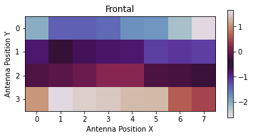
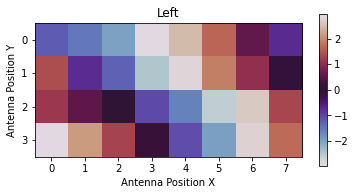
plot_array_phases(points_frontal_calibrated, 512, 8, "Frontal")
plot_array_phases(points_left_calibrated, 512, 8, "Left")
plot_array_phases(points_right_calibrated, 512, 8, "Right")

This time, we finally see the "textbook-like" phase pattern that we would expect for a uniform linear array (ULA):

• If the transmitter is in front of the array, the received phase decreases from the bottom to the top. This is because the antenna array is mounted at a hight of approximately 1.2m above the transmit antenna, so that the electromagnetic wave arrives earliest at the lowest row.
• If the transmitter is to the left or to the right of the array, in addition to the phase decrease from bottom to top, we can also see a decrease from the left to the right or inversely, respectively.

Classical Angle of Arrival (AoA) Estimation

But wait... doesn't this mean that, instead of applying neural networks to the task of transmitter position estimation, we could now just apply classical techniques? Well yes, it does! In the following, we are going to look at a very simple approach to this topic - note that much better, more advanced methods are available, such as the MUSIC algorithm. Within the scope of this tutorial, we only care about showing that classical AoA estimation is at all possible with DICHASUS data.

The following code snippets estimate the phase difference between antennas that are horizontal neighbors (for a small subcarrier range). Subsequently, this this measured phase difference is transformed to an AoA estimate using the well-known ULA AoA equation, i.e., \[ \Delta \varphi = \frac{2 \pi f_\mathrm{c}}{c} ~ d ~ \sin(\vartheta), \] where \( \Delta \varphi \) is the estimated phase difference between neighboring antennas, \( f_\mathrm{c} \) is the carrier frequency, \( c \) is the speed of light and \( \vartheta \) is the angle of arrival of the electromagnetic wave, measured relative to the perpendicular (see sketch).

# Apply phase calibration to complete dataset
dataset_calibrated = dataset.map(apply_calibration)

antenna_distance = 0.118

def estimate_frequency(samples):
	# Kay's Single Frequency Estimator:
	# S. Kay, "A fast and accurate single frequency estimator" in IEEE Transactions on Acoustics, Speech, and Signal Processing,
	# vol. 37, no. 12, pp. 1987-1990, Dec. 1989, doi: 10.1109/29.45547.
	N = len(samples)
	w = (3 / 2 * N) / (N**2 - 1) * (1 - ((np.arange(0, N - 1) - (N / 2 - 1)) / (N / 2))**2)
	return sum([w[t] * np.angle(np.conj(samples[t]) * samples[t + 1]) for t in np.arange(0, N - 1)])
		
def estimate_angles(dataset, subcarrier_start, subcarrier_count, fcarrier, bandwidth):
	positions = []
	angle_estimates = []
			
	for csi, pos in dataset:
		subcarriers = csi.shape[1]
		csi_mean = tf.math.reduce_sum(csi[:,subcarrier_start:subcarrier_start + subcarrier_count], axis = 1).numpy()
		wavelength = 299792458 / (fcarrier + bandwidth * (-subcarriers / 2 + subcarrier_start + subcarrier_count / 2) / subcarriers)
		phase_diff = np.mean([estimate_frequency(csi_mean[row]) for row in assignments])
		wavelength_diff = phase_diff * wavelength / antenna_distance / (2 * np.pi)
		
		angle_estimate = None
		if wavelength_diff <= -1:
			angle_estimate = -np.pi / 2
		elif wavelength_diff >= 1:
			angle_estimate = np.pi / 2
		else:
			angle_estimate = np.arcsin(wavelength_diff)
		
		positions.append(pos.numpy())
		angle_estimates.append(angle_estimate)
				
	return np.vstack(positions), np.hstack(angle_estimates)

Let's generate and plot some phase estimates! This may take a short while to compute.

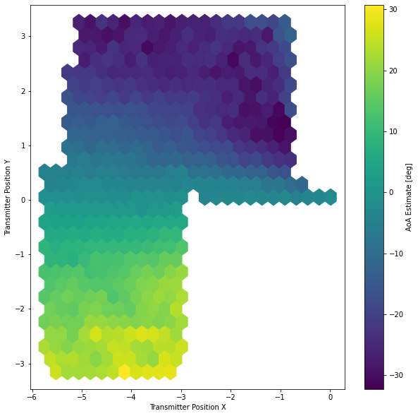
positions, angle_estimates = estimate_angles(dataset_calibrated, 512, 520, 1.272e9, 50e6)

plt.figure(figsize=(10,10))
plt.hexbin(positions[:,0], positions[:,1], C = np.rad2deg(angle_estimates), gridsize = 25)
plt.xlabel("Transmitter Position X")
plt.ylabel("Transmitter Position Y")
plt.colorbar(label = "AoA Estimate [deg]")
plt.show()

Remember that, in our dataset, the antenna array is located at \( (x, y) = (0, 0) \) and points in the negative \( x \) direction. The diagram that is generated is pretty convincing: We can clearly see the color gradient from the steep incident angles to the right of the antenna array (dark blue) to the angles on the left of the array (yellow).

Based on the position label of every datapoint, we can also compute an "ideal" AoA value for every datapoint and compare estimate and ideal value. Let's plot this estimation error in a histogram.

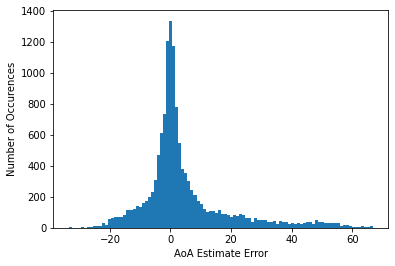
true_angles = np.arctan2(-positions[:,1], -positions[:,0] + 0.2)
est_error = np.rad2deg(np.angle(np.exp(1.0j * angle_estimates) * np.conj(np.exp(1.0j * true_angles))))
plt.xlabel("AoA Estimate Error")
plt.ylabel("Number of Occurences")
plt.hist(est_error, bins = 100)
plt.show()
print("MAE:", np.mean(np.abs(est_error)), "degrees")

Looking at a histogram of the AoA estimation error, we see that for most datapoints, the error is somewhere below \( 10^\circ \). In fact, the mean absolute error (MAE) we obtain is \( 9^\circ \). While this is worse than what we could have achieved using a neural network-based approach (typically \( 3^\circ - 5^\circ\) MAE), it clearly shows that classical AoA estimation is possible.

Conclusion

The results obtained in this tutorial show that the channel measurements performed with DICHASUS indeed reflect the physical reality. We also saw that the calibration of static phase and time offsets, which naturally occur due to the reference transmitter architecture, is absolutely crucial.

This kind of offset compensation is only relevant for classical signal processing methods though. When applying deep learning to DICHASUS datasets, neural networks will automatically learn all offsets in the training data and, since the offset are constant, account for the learned biases during inference. In fact, deep learning methods do not even need to know the physical setup of antennas. It is reassuring to see, though, that after careful calibration, classical methods can reach performance that is comparable to deep learning-based approaches for typical regression problems.

Licensing and Authors

The calibration parameters (phase offset and sampling time offset) for the datasets are provided courtesy of Phillip Stephan, who investigated the offset estimation method based on the line-of-sight component of the main transmitter signal. We intend to publish more information about this method in the future.

All our datasets are licensed under the CC-BY license, i.e., you are free to use them for whatever you like as long as you reference us in your publications. All code in this tutorial is CC0-licensed. This tutorial was written by Florian Euchner.