DICHASUS - Timestamp / Triplet-Based Channel Charting

Updated Tutorial Available

Based on insights from research published by our friends at Fraunhofer IIS and by ourselves (among many other influential publications), we developed a significantly improved Channel Charting technique. You can learn about this technique in our new tutorial on dissimilarity metric-based Channel Charting:

Read New Tutorial

Regardless, we keep this tutorial on timestamp/triplet-based Channel Charting online for the time being. We believe that this tutorial reflects one Channel Charting method that was the State-of-the-Art in the summer of 2022.

What is Channel Charting?

Thanks to global navigation satellite systems, your phone can tell you your location and reliably guide you to your destiation. Well, except if you are indoors or in an urban canyon of course, then you are on your own. And, sure it will drain your battery a bit faster. It will also take a few moments until your phone has picked up signals from sufficiently many satellites to localize you. Is this really the best technology can do?

We believe that, by leveraging future massive MIMO deployments in 5G and beyond in a process known as "Channel Charting", there is still room for enhancing geolocation services. Massive MIMO is a crucial technology for improving the spectral efficiency of wireless telecommunication systems through spatial multiplexing and will likely be deployed in the form of 5G base stations. With massive MIMO, the base station collects so-called channel state information (CSI) at every receiver antenna, from which the base station can infer properties like angles of arrival, reflections and propagation delays. While this is essential for ensuring the functionality of massive MIMO, CSI does not necessarily have to be stored and analyzed. But, what if we did just that, can we localize end users at the base station just from CSI? Well, sure! It has been shown that CSI-based user localization is possible (we have a tutorial on that!), at least with supervised machine learning methods such as CSI fingerprinting. These approaches, however, require "ground truth" position labels for the transmitter position, which are usually not available. Channel Charting, on the other hand, is a self-supervised learning technique which aims to create a virtual map of high-dimensional CSI. Therefore, Channel Charting is not dependent on the availability of position labels, which is a huge advantage over fingerprinting.

While faster and more reliable personal navigation will be the most visible advantage for end users, asset tracking and radio access network (RAN) management tasks will benefit even more significantly: Asset tracking, because embedding GNSS (e.g., GPS) receivers into trackers is often infeasible: A GNSS receiver is more expensive than just a wide-area radio modem, it doesn't work inside warehouses and needs a lot of energy and hence does not last on a battery for long (especially if the device is usually in sleep mode, and needs up to a minute to obtain an accurate position estimate after waking up before going back to sleep). The mobile network itself will also benefit significantly from the availability of location information at the base station. For example, knowing location and velocity of a user will allow the base station to predict the wireless channel into the future. In addition, the network will be able to plan handovers between base stations ahead of time ensuring seamless connectivity and prevent pilot contamination.

TL;DR - Video

This video (no audio) will explain Channel Charting in a more visual format:

DICHASUS Datasets for Channel Charting

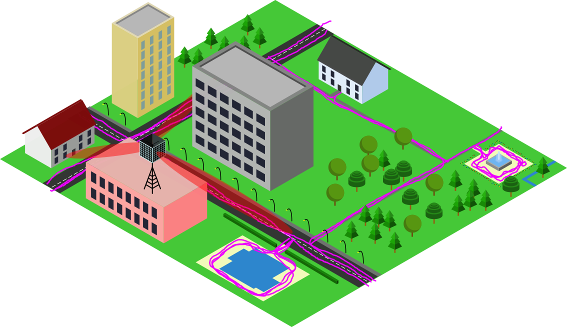
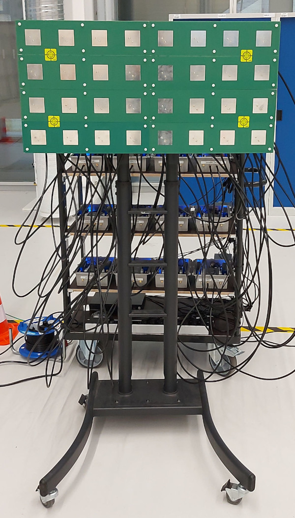
DICHASUS is not a "real" base station, but we can use channel sounder data to investigate the feasibility of Channel Charting in a real-world setup. The datasets are particularly suitable for Channel Charting research for several reasons:

Large datasets: Channel Charting needs lots of training data
Distributed massive MIMO: Channel Charting works better if there are several distributed, yet coherent antenna arrays. Want to test it with just one massive MIMO array? Just remove the others from the training set.
Real-world scenarios: If your algorithm works with DICHASUS datasets, you can show that it works in the real world (and not only in a simulator). The carrier frequency ranges that DICHASUS uses are close to the frequency range of real-world 4G/5G networks, so the chance that results will be reproducible on real distributed massive MIMO base stations is high.
Accurate "ground truth" positions: Since Channel Charting is unsupervised, you don't need these for training, but they are necessary for performance evaluations.

Of course, there are also some downsides to consider: Lower flexibility compared to simulations, only a limited number of datasets is available and the bandwidth could be better (even though real-world commercial wireless systems rarely offer much higher bandwidths).

Channel Charting Pipeline

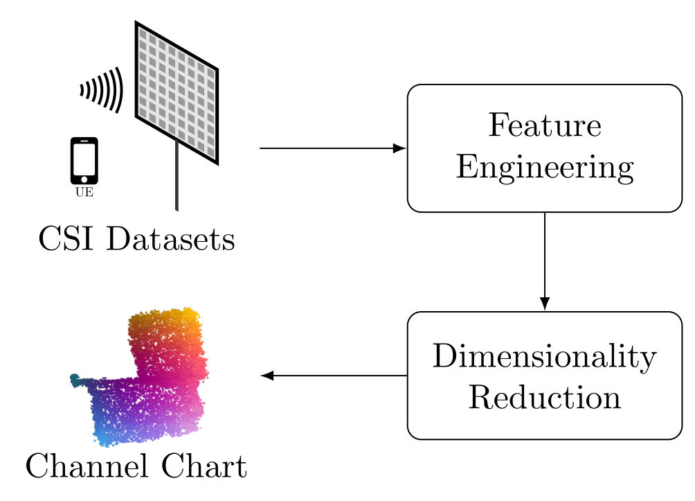
This tutorial will explain how to implement triplet neural network-based Channel Charting, which we consider to be the "State-of-the-Art" in 2022, with Python and TensorFlow. Our Channel Charting "pipeline" consists of two separate stages: First, we need to take the CSI datasets and extract some features from them, in a process known as Feature Engineering. The purpose of this step is to reduce the amount of data that the neural network has to process, and to provide the data to the neural network in a more suitable format. Second, we apply a dimensionality reduction technique to the resulting feature sets. Dimensionality reduction can either be some classical linear or nonlinear approach such as Principal Component Analysis (PCA) or Isomap, or, for better performance, a neural network-based method.

Neural Network-based Channel Charting: Forward Charting Function

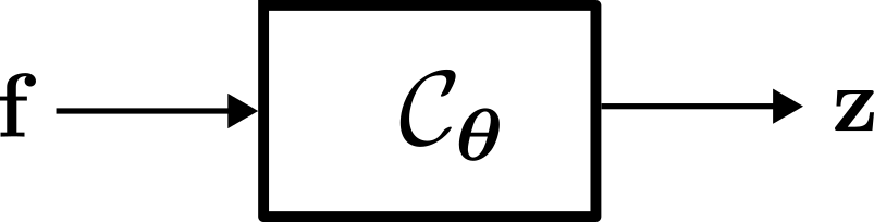
Regardless of the training method employed, the objective of neural network-based Channel Charting is to learn the so-called Forward Charting Function \( \mathcal C_{\boldsymbol \theta} \). The Forward Charting Function takes a feature vector \( \mathbf f \) as an input and directly outputs the position in the Channel Chart \( \mathbf z \). Once \( \mathcal C_{\boldsymbol \theta} \) has been found, this makes it very easy and efficient to infer Chart positions (this is not the case for other dimensionality reduction techniques!).

The \( \boldsymbol \theta \) in the subscript indicates that this function is parametrized by a parameter vector \( \boldsymbol \theta \), which contains the weights and biases of the neural network. The purpose of neural network training is to find suitable values for \( \boldsymbol \theta \).

But before we can do any of that, let's start with some basics about our datasets.

Downloading and Reading the CSI Dataset

For this tutorial, we use the dichasus-cf0x dataset collected by DICHASUS. This dataset contains CSI for \(B = 32\) receive antennas and for \(W = 1024\) OFDM subcarriers at \( N \) different transmitter positions. The transmitter is mounted on top of a robot, which follows some trajectory through the measurement area. The CSI at a particular time instant can be expressed as a matrix \(\mathbf H_n \in \mathbb C^{B \times W}\). The dataset is made up of data points that are 3-tuples of channel coefficients \( \mathbf{H}_{n} \in \mathbb C^{B \times W} \), ground truth positions \( \mathbf{x}_n \in \mathbb{R}^D \) and timestamps \( t_n \in \mathbb R \): \[ \text{Dataset:} \quad \left\{ (\mathbf{H}_{n}, \mathbf x_n, t_n) \right\}_{n = 1, \ldots, N} \] The ground truth positions (which are really only for evaluation purposes, they are not used for training!) are measured with a tachymeter robotic total station, a very precise instrument that tracks the robot's antenna with a laser with at least centimeter-level accuracy.

DICHASUS uses a reference transmitter for synchronization, which entails that measured phases may exhibit constant offsets caused by the specific channel between reference transmitter and receive antenna. Luckily, we computed these offsets for each DICHASUS dataset and made them available for download. The datasets themselves are provided in the TFRecords file format, which makes loading them with TensorFlow particularly simple. Obviously, the more training data we have, the better the channel chart gets. To save some disk and RAM space, we will settle for just 3 robot round trips in the following: dichasus-cf02.tfrecords, dichasus-cf03.tfrecords and dichasus-cf04.tfrecords:

!mkdir dichasus
!wget -nc --content-disposition https://darus.uni-stuttgart.de/api/access/datafile/:persistentId?persistentId=doi:10.18419/darus-2854/8 -P dichasus # dichasus-cf02
!wget -nc --content-disposition https://darus.uni-stuttgart.de/api/access/datafile/:persistentId?persistentId=doi:10.18419/darus-2854/9 -P dichasus # dichasus-cf03
!wget -nc --content-disposition https://darus.uni-stuttgart.de/api/access/datafile/:persistentId?persistentId=doi:10.18419/darus-2854/10 -P dichasus # dichasus-cf04
!wget -nc https://dichasus.inue.uni-stuttgart.de/datasets/data/dichasus-cf0x/reftx-offsets-dichasus-cf02.json -P dichasus
!wget -nc https://dichasus.inue.uni-stuttgart.de/datasets/data/dichasus-cf0x/reftx-offsets-dichasus-cf03.json -P dichasus
!wget -nc https://dichasus.inue.uni-stuttgart.de/datasets/data/dichasus-cf0x/reftx-offsets-dichasus-cf04.json -P dichasus

Next, we load the TFRecords files with TensorFlow and apply the offset compensation to the CSI as described in our offset compensation tutorial. To reduce the number of datapoints, we will only use every 2^nd datapoint for training and plotting (it is nevertheless important to load multiple robot round trips, since these provide diversity in the types of trajectories!).

import matplotlib.pyplot as plt
import tensorflow as tf
import numpy as np
import json

ANTENNACOUNT = 32

def load_and_calibrate(path, offset_path):
	offsets = None
	with open(offset_path, "r") as offsetfile:
		offsets = json.load(offsetfile)
	
	def record_parse_function(proto):
		record = tf.io.parse_single_example(
			proto,
			{
				"csi": tf.io.FixedLenFeature([], tf.string, default_value=""),
				"pos-tachy": tf.io.FixedLenFeature([], tf.string, default_value=""),
				"time": tf.io.FixedLenFeature([], tf.float32, default_value=0),
			},
		)

		csi = tf.ensure_shape(tf.io.parse_tensor(record["csi"], out_type=tf.float32), (ANTENNACOUNT, 1024, 2))
		csi = tf.complex(csi[:, :, 0], csi[:, :, 1])
		csi = tf.signal.fftshift(csi, axes=1)

		position = tf.ensure_shape(tf.io.parse_tensor(record["pos-tachy"], out_type=tf.float64), (3))
		time = tf.ensure_shape(record["time"], ())

		return csi, position[:2], time

	def apply_calibration(csi, pos, time):
		sto_offset = tf.tensordot(tf.constant(offsets["sto"]), 2 * np.pi * tf.range(tf.shape(csi)[1], dtype = np.float32) / tf.cast(tf.shape(csi)[1], np.float32), axes = 0)
		cpo_offset = tf.tensordot(tf.constant(offsets["cpo"]), tf.ones(tf.shape(csi)[1], dtype = np.float32), axes = 0)
		csi = tf.multiply(csi, tf.exp(tf.complex(0.0, sto_offset + cpo_offset)))

		return csi, pos, time

	return tf.data.TFRecordDataset(path).map(record_parse_function, num_parallel_calls = tf.data.AUTOTUNE).map(apply_calibration, num_parallel_calls = tf.data.AUTOTUNE)

inputpaths = [
	{
		"tfrecords" : "dichasus/dichasus-cf02.tfrecords",
		"offsets" : "dichasus/reftx-offsets-dichasus-cf02.json"
	},
	{
		"tfrecords" : "dichasus/dichasus-cf03.tfrecords",
		"offsets" : "dichasus/reftx-offsets-dichasus-cf03.json"
	},
	{
		"tfrecords" : "dichasus/dichasus-cf04.tfrecords",
		"offsets" : "dichasus/reftx-offsets-dichasus-cf04.json"
	}
]

training_set = load_and_calibrate(inputpaths[0]["tfrecords"], inputpaths[0]["offsets"])

for path in inputpaths[1:]:
	training_set = training_set.concatenate(load_and_calibrate(path["tfrecords"], path["offsets"]))

# Decimate dataset: Use only every 2nd datapoint (to reduce number of points)
training_set = training_set.enumerate().filter(lambda idx, value : (idx % 2 == 0))
training_set = training_set.map(lambda idx, value : value)

Feature Engineering

def average_over_subcarriers(csi, pos, time):
	csi = tf.reduce_mean(csi[:, 508:516], axis=1)
	return csi, pos, time

training_set = training_set.map(average_over_subcarriers, num_parallel_calls = tf.data.AUTOTUNE)

def scale_r2m(csi, pos, time):
	beta = 1 + 1 / 16
	
	second_moment = tf.tensordot(csi, tf.math.conj(csi), axes=0)
	csi = tf.constant(ANTENNACOUNT**(beta - 1), dtype = tf.complex64) / tf.math.pow(tf.norm(second_moment, ord = "fro", axis = (0, 1)), beta) * second_moment
	csi = tf.squeeze(tf.reshape(csi, (1, ANTENNACOUNT * ANTENNACOUNT)), axis = 0)
	csi = tf.math.real(csi)

	return csi, pos, time

training_set = training_set.map(scale_r2m, num_parallel_calls = tf.data.AUTOTUNE)

We apply a first pre-processing step by averaging each CSI vector over eight subcarriers in the center of the considered bandwidth as \[ \mathbf{\overline{h}}_n = \frac{1}{8}\sum_{w=508}^{515} \left[\mathbf{H}_{n}\right]_{b, w} \in \mathbb{C}^{32} \]

The reason for this is to reduce the dimensionality of the CSI while keeping the large-scale fading characteristics of the channel. We do lose some information here (most notably, antenna-specific time delays), so feel free to improve this step if you have good hardware accelerators for training. We further apply a method described in the initial paper on Channel Charting, namely we compute the scaled raw second moment (R2M) \[ \mathbf f_n = \mathrm{Re} \left\{ \mathrm{vec} \left\{ \frac{B^{\beta - 1}}{\left\lVert \mathbf{\overline{h}}_n ~ \mathbf{\overline{h}}_n^\mathrm{H} \right\rVert^\beta_\mathrm{F}} ~~ \mathbf{\overline{h}}_n ~ \mathbf{\overline{h}}_n^\mathrm{H} \right\} \right\}. \] By vectorization and only considering its real part (again, we are losing information here, space for improvement!), we obtain the feature vector \(\mathbf{f}_n \in \mathbb R^{B^2}\), which we use for training. After feature engineering, our training dataset looks as follows: \[ \text{Dataset:} ~~~ \left\{ (\mathbf{f}_{n}, \mathbf x_n, t_n) \right\}_{n = 1, \ldots, N} \]

At this point, if your RAM is large enough for all TFRecords to fit inside, it might be a good idea to cache the training set so that all the subsequent training and evaluation steps will be quicker. If your RAM is small (or you want to train on really huge training sets), don't worry: The datasets can also remain on disk storage, and the training code will load batches of triplets from there when needed.

# If you have enough RAM...
training_set = training_set.cache()

Visualizing the Dataset

Now that we have loaded the TFRecords dataset and applied some feature engineering stages, let's have a look at what the dataset actually looks like. For this, we plot the afforementioned ground truth positions. Additionally, we store a mapping from datapoint timestamp to the index in the dataset in a Python dictionary called timestamp_index_map and sort this dictionary by timestamp (the dataset is not guaranteed to be sorted in any way!). The purpose of this list will become apparent later on.

Running this code segment may take a lot of time - this is because all of the previous code segments only added processing steps to TensorFlow's compute graph. It is only in the following processing step, that the datapoints are actually read from disk and feature engineering is applied.

# This may take a long time, since TensorFlow has to load the dataset from disk!
groundtruth_positions = []
timestamp_index_map = dict()

for index, data in enumerate(training_set):
	groundtruth_positions.append(data[1].numpy())
	timestamp_index_map[data[2].numpy()] = index

timestamp_index_map = dict(sorted(timestamp_index_map.items()))
groundtruth_positions = np.asarray(groundtruth_positions)

We use the plot_colorized function to plot the ground truth positions. It produces a scatter plot, where each point in the scatter plot is assigned a color according to its ground truth position. We can later reuse this function to plot the channel chart with the same colorization.

def plot_colorized(positions, title = None):
	# Generate RGB colors for datapoints
	center_point = np.zeros(2, dtype = np.float32)
	center_point[0] = 0.5 * (np.min(groundtruth_positions[:, 0], axis = 0) + np.max(groundtruth_positions[:, 0], axis = 0))
	center_point[1] = 0.5 * (np.min(groundtruth_positions[:, 1], axis = 0) + np.max(groundtruth_positions[:, 1], axis = 0))
	NormalizeData = lambda in_data : (in_data - np.min(in_data)) / (np.max(in_data) - np.min(in_data))
	rgb_values = np.zeros((groundtruth_positions.shape[0], 3))
	rgb_values[:, 0] = 1 - 0.9 * NormalizeData(groundtruth_positions[:, 0])
	rgb_values[:, 1] = 0.8 * NormalizeData(np.square(np.linalg.norm(groundtruth_positions - center_point, axis=1)))
	rgb_values[:, 2] = 0.9 * NormalizeData(groundtruth_positions[:, 1])

	# Plot datapoints
	plt.figure(figsize=(6, 6))
	if title is not None:
		plt.suptitle(title, fontsize=16)
	plt.scatter(positions[:, 0], positions[:, 1], c = rgb_values, s = 5)

plot_colorized(groundtruth_positions, title="Ground Truth Positions")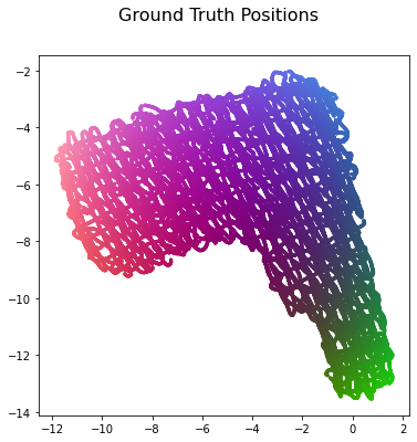

Triplet-Based Dimensionality Reduction

Now that we have loaded our CSI datasets and applied feature engineering, we are ready for the most important part of Channel Charting: the dimensionality reduction algorithm. Keeping in mind that Channel Charting is a self-supervised training method, we need to pretend that we don't know the ground truth positions. The channel chart should maintain the local geometry of the transmitter positions, i.e., any two positions \( \mathbf{x}, \mathbf{x'} \in \mathbb{R}^D \) that are close to each other in the real world should also be close to each other in the channel chart, with \( \mathbf{z}, \mathbf{z'} \in \mathbb{R}^{D'} \) being the corresponding points in the channel chart. In other words, the condition \[ \mathrm d_\mathrm{z} \left( \mathbf{z}, \mathbf{z'} \right) \approx \mathrm d_\mathrm{x} \left( \mathbf{x}, \mathbf{x'} \right) \] should be satisfied for any neighboring data points, with \( \mathrm d_\mathrm{z} \left( \cdot, \cdot \right) \) and \( \mathrm d_\mathrm{x} \left( \cdot, \cdot \right) \) being appropriately defined dissimilarity measures. Finding such a dissimilarity measure is not trivial, as the Euclidean distance is a poor representation for high-dimensional data. This problem is elegantly circumvented by the triplet-based dimensionality reduction technique, which takes timestamps as side information into account. Its principle is simple: Triplets of CSI samples are selected based on their timestamps. Each triplet consists of a randomly selected anchor point and a positive sample which is closer to the anchor point in time than a third sample, which is called the negative sample. Since anchor and positive sample are close to each other in time, it is very likely that they are also close to each other in space, the converse holds for anchor and negative sample. These Triplets can then be processed by a special neural-network-structure called "Triplet Network" with a special type of loss function called triplet loss.

Triplet Loss

Triplet loss ensures that training leads to the positive sample getting closer to the anchor than the negative sample in the channel chart by penalizing output triplets where the negative sample is closer to the anchor point than the positive sample. Let \( \mathcal T \) be the set of triplets, where a single triplet is given by the indices \( (i, j, k) \in \mathcal T \) of anchor point (\( i \)), positive sample (\( j \)) and negative sample (\( k \)) in the dataset. We define and implement the loss function as \[ \mathcal{L}=\frac{1}{\mathcal{|T|}}\sum_{\left(i,j,k\right)\in \mathcal{T}}\max\left(\Vert\mathbf{z}_i-\mathbf{z}_j\Vert-\Vert\mathbf{z}_i-\mathbf{z}_k\Vert+M,0\right). \]

def triplet_loss(y_true, y_pred):
	anchor, positive, negative = (y_pred[:, :CC_DIMENSIONALITY], y_pred[:, CC_DIMENSIONALITY : 2 * CC_DIMENSIONALITY], y_pred[:, 2 * CC_DIMENSIONALITY :])
	positive_dist = tf.reduce_mean(tf.square(anchor - positive), axis = 1)
	negative_dist = tf.reduce_mean(tf.square(anchor - negative), axis = 1)
			
	return tf.maximum(positive_dist - negative_dist + 1, 0.0)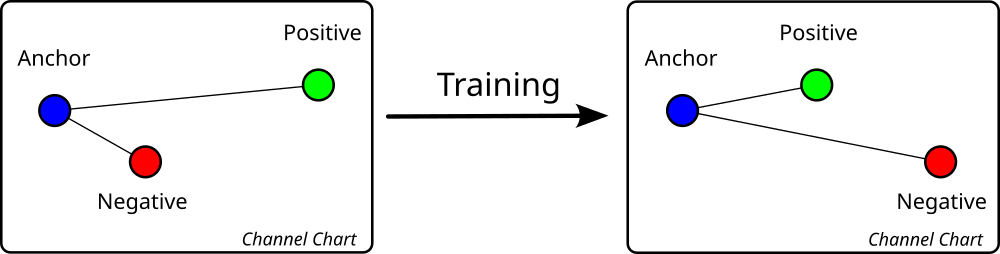

Triplet Selection

For training, we need to create a large set of triplets \(\left(i,j,k\right)\in \mathcal{T}\). Ideally, these triplets would be selected such that the condition \[ \lVert \mathbf{x}_i - \mathbf{x}_j \rVert \leq \lVert \mathbf{x}_i - \mathbf{x}_k \rVert \] holds for their respective ground truth positions \( \mathbf{x}_i \), \( \mathbf{x}_j \) and \( \mathbf{x}_k \). Using ground truth information would be cheating though, we are looking for a self-supervised training method. But there is another crucial piece of information that is available at the base station that we can exploit: The CSI timestamps! Since the user travels with a finite velocity, we can assume that two CSI vectors measured within a short timeframe are likely to be close to each other. Consequently, we select the triplets based on their timestamps such that \[ \mathcal T = \{ \left(i, j, k \right): |t_j - t_i| \leq T_\mathrm{c} \}, \] with \( T_c \) being the maximum elapsed time between anchor point and positive sample.

Admittedly, the following Python code, which generates a set of triplets \( \mathcal T \) provided \( T_\mathrm{c} \) is not pretty - but it is efficient. The idea here is that we only operate on timestamps and indices in the dataset and only once we have decided which triplets to load from the training set, we iterate once over training_set and collect all the CSI features that we are interested in. This way, the dataset can remain on disk if our available RAM is limited.

More precisely, we take the following steps to obtain \( \mathcal T \) from the training set:

Given the particular elapsed time threshold \( T_\mathrm{c} \), generate a lookup table that, for every potential anchor point \( i \), contains all suitable positive sample indices \( j \). That is, all sample indices \( i \) such that \( |t_i - t_j| \leq T_\mathrm{c} \). Since timestamp_index_map is sorted, this lookup table can be computed very efficiently in a single iteration over timestamp_index_map.
Based on the lookup table, randomly generate a list of triplets \( \mathcal T \). The negative sample index \( k \) is drawn randomly from the set of all datapoints. By the sheer number of datapoints, is unlikely that \( \mathbf x_k \) is closer to \( \mathbf x_i \) than \( \mathbf x_j \).
From \( \mathcal T \), generate a list of datapoint indices to load the CSI features for and also remember what sample (anchor / positive / negative) of which triplet(s) these features belong to.
Then, iterate over the dataset (on disk or, if cached, in RAM) only once and load all of the CSI features for all triplets.

For now, we only define some functions. We will call generate_triplets later for every batch of triplets to generate.

def generate_positive_sample_lookup(Tc = 1.5):
	lookup = dict()
	suitable_set = dict()
	candidate_iterator = iter(timestamp_index_map.items())
	next_suitable = next(candidate_iterator)

	for anchor_timestamp, anchor_index in timestamp_index_map.items():
		# Add additional later suitable datapoints to suitable_set
		while next_suitable[0] - anchor_timestamp < Tc:
			suitable_set.update((next_suitable,))
			try:
				next_suitable = next(candidate_iterator)
			except StopIteration:
				break

		# Remove too early suitable datapoints from suitable_set
		outdated = []
		for timestamp in suitable_set.keys():
			if anchor_timestamp - timestamp > Tc:
				outdated.append(timestamp)
			else:
				for o in outdated:
					del suitable_set[o]
				break

		# For every potential anchor point, store lookup table of potential positive sample indices
		lookup[anchor_index] = set(suitable_set.values())
		
		# Set of suitable positive samples must not contain anchor itself
		lookup[anchor_index].remove(anchor_index)
		lookup[anchor_index] = list(lookup[anchor_index])

	return lookup

def generate_triplets(nr_of_triplets = 1000, Tc = 1.5):
    print("Generating lookup table for positive samples")
    positive_sample_lookup = generate_positive_sample_lookup(Tc)

    # Generate list of triplet containing *indices* of datapoints in dataset
    triplet_indices = []
    anchor_indices = list(positive_sample_lookup.keys())
    
    while len(triplet_indices) < nr_of_triplets:
        anchor = anchor_indices[np.random.randint(len(anchor_indices))]
        
        # Must ensure that anchor point is not a loner and actually has some close positive samples
        if len(positive_sample_lookup[anchor]) < 1:
            continue

        positive = np.random.choice(positive_sample_lookup[anchor])
        negative = anchor_indices[np.random.randint(len(anchor_indices))]
        
        triplet_indices.append((anchor, positive, negative))

    # Iterate over dataset (on hard drive storage) and load relevant CSI data to "triplets" list (in RAM)
    datapoints_to_load = dict()
    for target, indices in enumerate(triplet_indices):
        for sample in range(3):
            if indices[sample] not in datapoints_to_load:
                datapoints_to_load[indices[sample]] = []
            datapoints_to_load[indices[sample]].append((target, sample))

    datapoints_to_load = dict(sorted(datapoints_to_load.items()))

    anchors = [None for i in range(len(triplet_indices))]
    positives = [None for i in range(len(triplet_indices))]
    negatives = [None for i in range(len(triplet_indices))]

    print("Loading batch of triplets from dataset (on disk or in RAM)")
    for index, data in enumerate(training_set):
        if index in datapoints_to_load:
            for target in datapoints_to_load[index]:
                if target[1] == 0:
                    anchors[target[0]] = data[0]
                elif target[1] == 1:
                    positives[target[0]] = data[0]
                elif target[1] == 2:
                    negatives[target[0]] = data[0]
    print("Finished loading triplet batch")

    return [tf.stack(anchors), tf.stack(positives), tf.stack(negatives)]

Neural Network Architecture

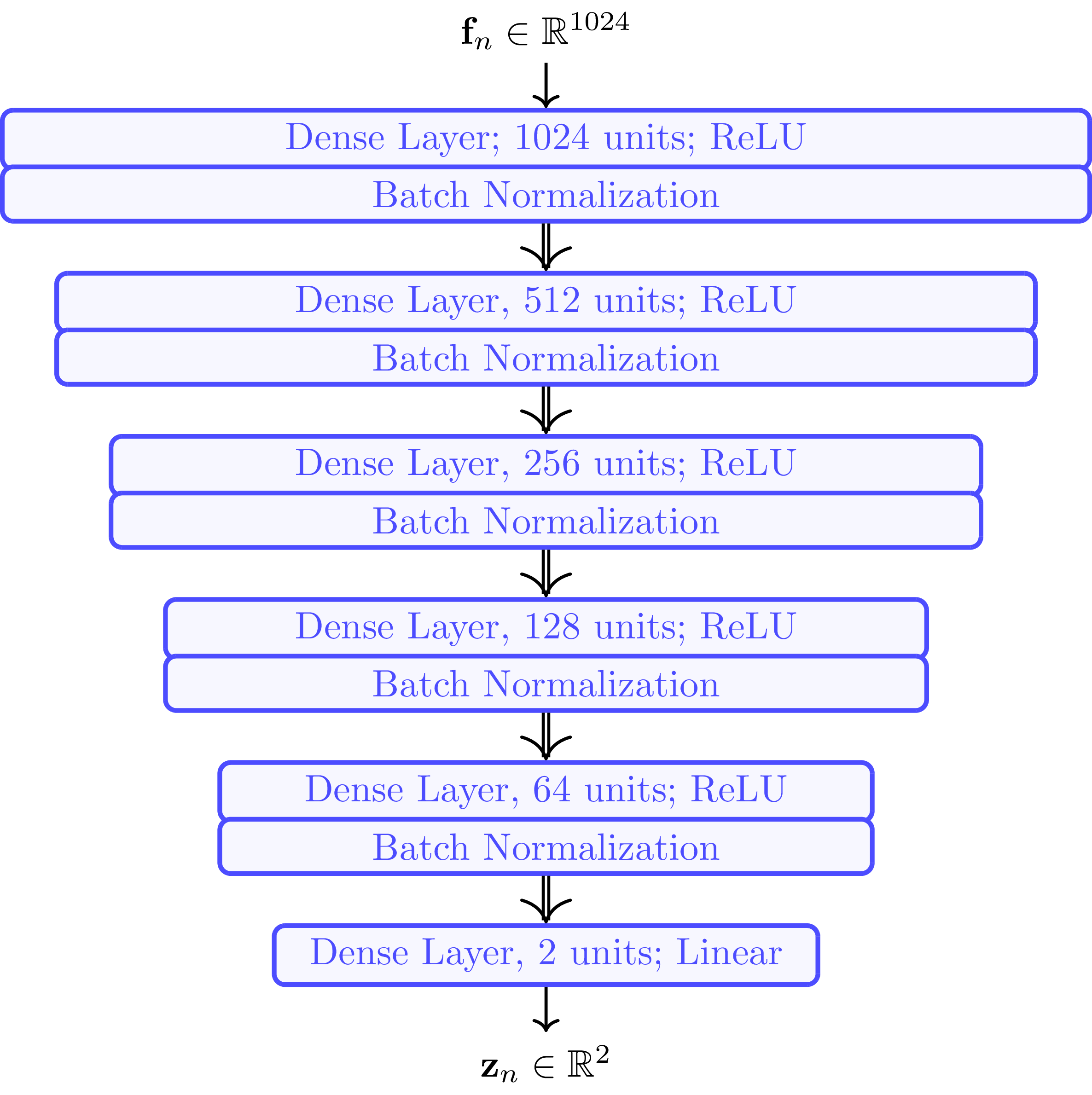
The DNN is trained to learn the Forward Charting Function \( \mathcal C_{\boldsymbol \theta} \), which maps the high-dimensional features to the low-dimensional points in the channel chart. The DNN itself is built from several dense layers followed by batch normalization layers. The input layer has \(1024\) neurons, matching the dimensionality of the input feature vector \( \mathbf f_n \) (\( B^2 = 32^2 = 1024 \)). Unsurprisingly, since the channel chart is \(2\)-dimensional, the output layer has only two neurons.

CC_DIMENSIONALITY = 2
embedding_model = tf.keras.models.Sequential(
	[
		tf.keras.layers.Dense(ANTENNACOUNT * ANTENNACOUNT, activation = "relu", input_shape = (ANTENNACOUNT * ANTENNACOUNT,)),
		tf.keras.layers.BatchNormalization(),
		tf.keras.layers.Dense(512, activation = "relu"),
		tf.keras.layers.BatchNormalization(),
		tf.keras.layers.Dense(256, activation = "relu"),
		tf.keras.layers.BatchNormalization(),
		tf.keras.layers.Dense(128, activation = "relu"),
		tf.keras.layers.BatchNormalization(),
		tf.keras.layers.Dense(64, activation = "relu"),
		tf.keras.layers.BatchNormalization(),
		tf.keras.layers.Dense(CC_DIMENSIONALITY, activation = "linear"),
	]
)

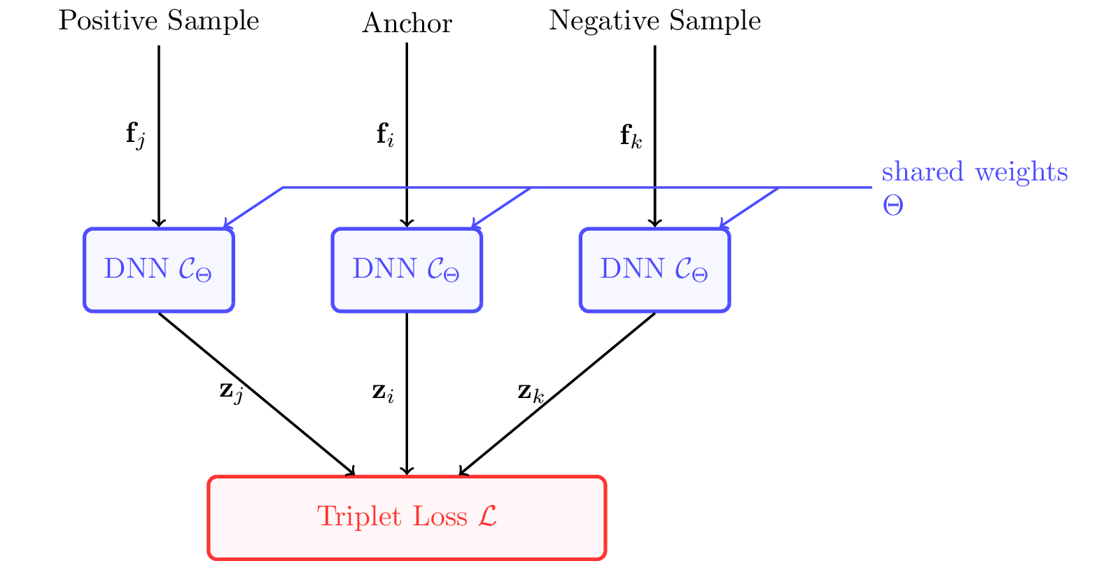
For training, we need to embed the DNN \( \mathcal C_{\boldsymbol \theta} \) into a triplet neural network. The three feature vectors of a triplet are each fed into the DNN, which then outputs the three corresponding low-dimensional points. From the three output points, TensorFlow then computes gradients for backpropagation using our triplet loss.

input_anchor = tf.keras.layers.Input(shape=(ANTENNACOUNT * ANTENNACOUNT,))
input_positive = tf.keras.layers.Input(shape=(ANTENNACOUNT * ANTENNACOUNT,))
input_negative = tf.keras.layers.Input(shape=(ANTENNACOUNT * ANTENNACOUNT,))

embedding_anchor = embedding_model(input_anchor)
embedding_positive = embedding_model(input_positive)
embedding_negative = embedding_model(input_negative)

output = tf.keras.layers.concatenate([embedding_anchor, embedding_positive, embedding_negative], axis=1)
model = tf.keras.models.Model([input_anchor, input_positive, input_negative], output)

Neural Network Training

Finally, we are ready to train the DNN. The elapsed time threshold between anchor and positive sample decreases for every training batch (\(T_c = 5.5 \dots 3\)). The training itself is performed in eight sessions. In each session, a new dataset with \( 150\,000 \) triplets is generated, on which the DNN is trained for ten epochs. The learning rate decreases every few sessions, but the batch size remains at constant \( 8\,192 \). All of these hyperparameters are definitely subject to further optimization!

optimizer = tf.keras.optimizers.Adam()
model.compile(loss = triplet_loss, optimizer = optimizer)

batch_size = 8192
learning_rates = [1e-3, 1e-3, 1e-4, 1e-4, 1e-5, 1e-5, 1e-5, 1e-5]
T_c = 5

for l in range(len(learning_rates)):
	print("\nTraining Session ", l + 1, "\nT_c =", T_c)
	triplets = generate_triplets(150000, T_c)
	optimizer.learning_rate.assign(learning_rates[l])
	print("\nBatch Size: ", batch_size, "\nEpochs: ", 10, "\nLearning rate: ", learning_rates[l])
	model.fit(triplets, triplets, batch_size = batch_size, steps_per_epoch = int(len(triplets[0]) / batch_size), epochs = 10)

Plotting the Channel Chart

Now we can let the trained DNN \( \mathcal C_{\boldsymbol \theta} \) predict points in the channel chart given CSI features from the training set. But wait! Isn't it common in machine learning tasks to do this on a test set? In our case, we applied an unsupervised learning technique, so the ground truth information is not known to the DNN. Therefore, and since the real goal of Channel Charting is to learn a sparse (low-dimensional) representation of CSI, we will use the training set here. Let's see what the DNN predicts if we feed it with the CSI feature vectors \( \mathbf f_n \).

channel_chart_positions = []
	
for csi, pos, timestamp in training_set.batch(1000):
	channel_chart_positions.append(embedding_model.predict(csi))

channel_chart_positions = np.vstack(channel_chart_positions)

plot_colorized(channel_chart_positions, title = "Channel Chart")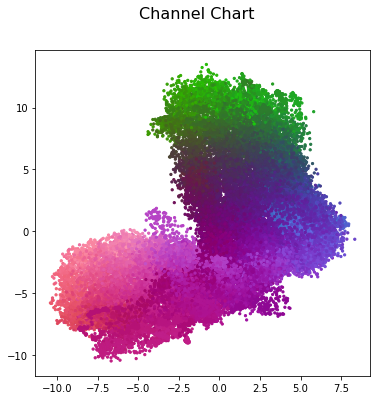

Thanks to the colorization (remember, colors are assigned according to the ground truth positions) we can directly see that CSI vectors measured at similar user positions are also placed close to each other in the channel chart. The global structure of the positions is also preserved to a certain degree.

Performance Evaluation

The goal of Channel Charting is to preserve the local geometry of the UE positions, and ideally the global geometry as well. However, we can't compare the channel chart with the ground truth positions using metrics such as mean squared error: If the geometry of the transmitter positions was preserved perfectly, since we don't have any known reference locations, the channel chart can always only match the real positions down to some linear transformation (i.e., some combination of rotation, scaling and / or reflection). Therefore, we need to find other metrics to measure the performance of the learned forward charting function. Channel Charting literature employs performance metrics that are also commonly used in other dimensionality reduction tasks. We use three different metrics out of them to evaluate our channel charts:

Continuity (CT) and Trustworthiness (TW), both normalized to range \( [0, 1] \), are two measures for the preservation of local neighborhoods. A high CT indicates that many neighborhood relationships in physical space are preserved in the channel chart. A high TW value, on the other hand, indicates that the channel chart does not contain many additional false neighborhood relationships, i.e., ones which are not present in the physical space. Trustworthiness is already implemented in the scikit-learn package. We implement continuity based on this implementation of the trustworthiness.
Kruskal Stress (KS) is a measure for the preservation of the global channel chart structure. It is also bounded to the range \( [0,1] \), but this time with 0 indicating the best and 1 indicating the worst possible performance.

from sklearn.metrics import pairwise_distances
from sklearn.neighbors import NearestNeighbors
from sklearn import manifold
import random

# Continuity is identical to trustworthiness, except that original space and embedding space are flipped
def continuity(*args, **kwargs):
	args = list(args)
	args[0], args[1] = args[1], args[0]
	return manifold.trustworthiness(*args, **kwargs)

def kruskal_stress(X, X_embedded, *, metric="euclidean"):
	dist_X = pairwise_distances(X, metric = metric)
	dist_X_embedded = pairwise_distances(X_embedded, metric = metric)
	beta = np.divide(np.sum(dist_X * dist_X_embedded), np.sum(dist_X_embedded * dist_X_embedded))

	return np.sqrt(np.divide(np.sum(np.square((dist_X - beta * dist_X_embedded))), np.sum(dist_X * dist_X)))

Computing and storing pairwise distances for the CT, TW and KS metrics is both memory-intensive and computationally expensive. We therefore compute these metrics on a randomly picked subset of datapoints, consisting of only every tenth datapoint:

subset_indices = random.sample(range(len(groundtruth_positions)), len(groundtruth_positions) // 10)

groundtruth_positions_subset = groundtruth_positions[subset_indices]
channel_chart_positions_subset = channel_chart_positions[subset_indices]

ct_train = continuity(groundtruth_positions_subset, channel_chart_positions_subset, n_neighbors = int(0.05 * len(groundtruth_positions_subset)))
tw_train = manifold.trustworthiness(groundtruth_positions_subset, channel_chart_positions_subset, n_neighbors = int(0.05 * len(groundtruth_positions_subset)))
ks_train = kruskal_stress(groundtruth_positions_subset, channel_chart_positions_subset)

metrics_channel_chart_train = np.around(np.array([ct_train, tw_train, ks_train]), 4)

print("CT: {} \nTW: {} \nKS: {}".format(*metrics_channel_chart_train))

Obviously, continuity and trustworthiness are close to 1, and the kruskal stress is close to 0. This confirms our first impression of the channel chart to be a locally, as well as globally reasonable representation of the radio environment.

>> CT: 0.9736
>> TW: 0.957
>> KS: 0.2596

Conclusion

We successfully applied triplet-based Channel Charting to a DICHASUS dataset. The key takeaways are:

Triplet-based Channel Charting is feasible on real CSI measured by DICHASUS, exploiting timestamp metadata.
Performance, as measured by the evaluation metrics Continuity, Trustworthiness and Kruskal Stress, is acceptable, but can be improved further using more training data, hyperparameter tuning or better training approaches.

A Note on Privacy

Last, but not least: If you read the whole tutorial all the way to the end, then you have certainly realized that Channel Charting technology means that the massive MIMO base station will know the location of the users in a much more fine-grained manner than is possible with today's base stations and their sector antennas. In my experience, Channel Charting researchers are very aware of the potential privacy implications. There are some very obvious benefits attached to Channel Charting (outlined in the introduction), but there is also potential for abuse. With all the skepticism about 5G and mobile networks in general, we believe it is important to transparently publish and discuss the advantages and risks of this technology.

Licensing and Authors

All our datasets are licensed under the CC-BY license, i.e., you are free to use them for whatever you like as long as you reference us in your publications. All code in this tutorial is CC0-licensed. This tutorial was written by Phillip Stephan.